from phasic import (
Graph, with_ipv, GaussPrior, HalfCauchyPrior,
Adam, Adamelia, ExpStepSize, ExpRegularization, clear_caches,
clear_jax_cache, clear_model_cache,
StateIndexer, Property, PropertySet, set_log_level
) # ALWAYS import phasic first to set jax backend correctly
set_log_level('WARNING')
import numpy as np
import jax.numpy as jnp
import pandas as pd
from typing import Optional
import matplotlib.pyplot as plt
from matplotlib.colors import LogNorm
import seaborn as sns
%config InlineBackend.figure_format = 'svg'
from tqdm.auto import tqdm
from typing import Optional, Callable
from functools import partial
from itertools import combinations, combinations_with_replacement
all_pairs = partial(combinations_with_replacement, r=2)
from vscodenb import set_vscode_theme
np.random.seed(42)
set_vscode_theme()
sns.set_palette('tab10')
# set_log_level('DEBUG')Joint probability inference
Discrete feature joint probability
If you have access to marginal features like counts of mutations shared by your samples (singletons, doubletons etc.), You can compute the joint probability of such events exactly.
Coalescent
nr_samples = 4
indexer = StateIndexer(
lineage=[
Property('descendants', min_value=1, max_value=nr_samples),
]
)
@with_ipv([nr_samples]+[0]*(nr_samples-1))
def coalescent_1param(state):
transitions = []
for i, j in all_pairs(indexer.lineage):
p1 = indexer.lineage.index_to_props(i)
p2 = indexer.lineage.index_to_props(j)
same = int(i == j)
if same and state[i] < 2:
continue
if not same and (state[i] < 1 or state[j] < 1):
continue
new = state.copy()
new[i] -= 1
new[j] -= 1
descendants = p1.descendants + p2.descendants
k = indexer.lineage.props_to_index(descendants=descendants)
new[k] += 1
transitions.append([new, [state[i]*(state[j]-same)/(1+same)]])
return transitions
Step one is to construct the model graph.
graph = Graph(coalescent_1param)
graph.plot()
From the model graph we can now create an augmented discrete graph that allow us to compute joint probabilities. This graph is generated for this purpose only and does not otherwise represent the original model. The trick is to track all combinations of events. Each combination is represented by a state with the absorbing one as its only child making each of them the last state in a path through the graph. The probability of passing through one such state thus represents a joint probability. Because we cannot model infinitely many combinations of discrete events, we cap the number of allowed events and route all additional events to an infinite loop not contributing to any joint probability thus defining the distributions deficit.
mutation_rate = 1
joint_prob_graph = graph.joint_prob_graph(indexer, tot_reward_limit=2, mutation_rate=mutation_rate)
joint_prob_graph.vertices_length()39Note that the edges now have, not one, but two coefficients. The extra one holds a value scaling the mutation rate.
joint_prob_graph.param_length()2Update edge weights to make the model reflect our true parameter values:
true_theta = [7, mutation_rate]
joint_prob_graph.update_weights(true_theta)
joint_prob_graph.plot(nodesep=0.3)
Compute the joint probabilities:
joint_prob_table = joint_prob_graph.joint_prob_table()
joint_prob_table| descendants_1 | descendants_2 | descendants_3 | descendants_4 | prob | |
|---|---|---|---|---|---|
| t_vertex_index | |||||
| 9 | 0 | 0 | 0 | 0 | 0.621377 |
| 18 | 0 | 1 | 0 | 0 | 0.071919 |
| 20 | 1 | 0 | 0 | 0 | 0.151842 |
| 23 | 0 | 0 | 1 | 0 | 0.046028 |
| 30 | 0 | 2 | 0 | 0 | 0.013225 |
| 31 | 2 | 0 | 0 | 0 | 0.026469 |
| 32 | 1 | 0 | 1 | 0 | 0.018067 |
| 33 | 0 | 0 | 2 | 0 | 0.005114 |
| 34 | 1 | 1 | 0 | 0 | 0.016322 |
| 35 | 0 | 1 | 1 | 0 | 0.001918 |
Deficit:
(1 - joint_prob_table['prob'].sum()).item()0.02771995193202048Test data
For testing and demonstration purposes, we can sample observations from the model.
def sample_joint_observations(joint_prob_graph, theta, nr_observations=1000):
joint_prob_graph.update_weights(theta)
joint_prob_table = joint_prob_graph.joint_prob_table()
p = joint_prob_table['prob'] / joint_prob_table['prob'].sum()
p = p.to_numpy()
sample = np.random.choice(joint_prob_table.index.values, nr_observations, p=p)
observations = joint_prob_table.loc[sample, joint_prob_table.columns[:-1]].to_numpy().tolist()
return observationstrue_theta = [7, mutation_rate] # coalescent rate and mutation rate
observations = sample_joint_observations(joint_prob_graph, true_theta, nr_observations=1000)
observations[:5][[0, 0, 0, 0], [2, 0, 0, 0], [1, 0, 0, 0], [0, 0, 0, 0], [0, 0, 0, 0]]For real data, make sure to only to include observations that are possible under the model:
modelled_obs = joint.loc[sample, joint.columns[:-1]].to_numpy().tolist()
allowed_observations = set(tuple(x) for x in modelled_obs)
observations = [o for o in observations if tuple(o) in allowed_observations]
observations = np.array(observations)
observationsConvert to the corresponding indices in the joint graph:
#set_log_level('DEBUG')
svgd = joint_prob_graph.svgd(
observations,
fixed=[(1, mutation_rate)], # Fix theta[1] (mutation) at actual mutation_rate value
n_iterations=200,
# prior=GaussPrior(ci=[1, 5]),
# optimizer=Adamelia(learning_rate=0.2),
learning_rate = ExpStepSize(first_step=0.05, last_step=0.005, tau=30.0),
# regularization=ExpRegularization(first_reg=10.0, last_reg=0.1, tau=20.0),
)svgd.summary(ci_method='hpd', ci_level=0.95)Parameter Fixed MAP Mean SD HPD 95% lo HPD 95% hi
0 No 7.5159 7.8857 1.5010 5.6309 11.2284
1 Yes 1.0000 NA NA NA NA
Particles: 40, Iterations: 200svgd.plot_ci(ci_method='hpd')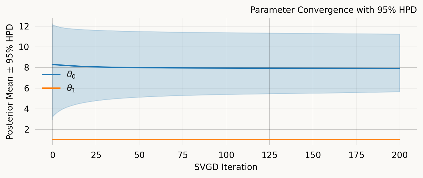
svgd.plot_convergence()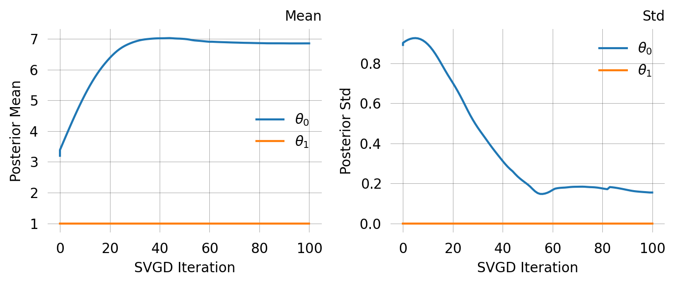
svgd.plot_trace()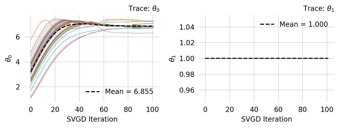
ARG
# create state space for two-locus model
nr_samples = 3
indexer = StateIndexer(
descendants=[
Property('loc1', min_value=0, max_value=nr_samples),
Property('loc2', min_value=0, max_value=nr_samples)
]
)
# initial state with all lineages having one descendant at both loci
initial = [0] * indexer.state_length
initial[indexer.descendants.props_to_index(loc1=1, loc2=1)] = nr_samples
@with_ipv(initial)
def two_locus_arg_2param(state, indexer=None):
transitions = []
if state.sum() <= 1: return transitions
for i in range(indexer.state_length):
if state[i] == 0: continue
props_i = indexer.descendants.index_to_props(i)
for j in range(i, indexer.state_length):
if state[j] == 0: continue
props_j = indexer.descendants.index_to_props(j)
same = int(i == j)
if same and state[i] < 2:
continue
if not same and (state[i] < 1 or state[j] < 1):
continue
child = state.copy()
child[i] -= 1
child[j] -= 1
des_loc1 = props_i.loc1 + props_j.loc1
des_loc2 = props_i.loc2 + props_j.loc2
if des_loc1 <= nr_samples and des_loc2 <= nr_samples:
child[indexer.descendants.props_to_index(loc1=des_loc1, loc2=des_loc2)] += 1
transitions.append([child, [state[i]*(state[j]-same)/(1+same), 0]])
if state[i] > 0 and props_i.loc1 > 0 and props_i.loc2 > 0:
child = state.copy()
child[i] -= 1
child[indexer.descendants.props_to_index(loc1=0, loc2=props_i.loc2)] += 1
child[indexer.descendants.props_to_index(loc1=props_i.loc1, loc2=0)] += 1
transitions.append([child, [0, state[i]]])
# transitions.append([child, [0, 1]])
return transitionsgraph = Graph(two_locus_arg_2param, indexer=indexer,
# graph_cache=True,
# cache_trace=True
)
graph.vertices_length()32graph.plot(nodesep=0.5, wrap=False)
mutation_rate = 1
joint_prob_graph = graph.joint_prob_graph(indexer,
reward_only=['loc1', 'loc2'],
reward_limit=1,
tot_reward_limit=2,
mutation_rate=mutation_rate
)true_theta = [10, 1, mutation_rate] # coalescent, recombination, and mutation rate
observations = sample_joint_observations(joint_prob_graph, true_theta, nr_observations=1000)
observations[:5][[0, 0, 0, 0, 0, 0, 0, 0],
[0, 0, 1, 0, 0, 0, 1, 0],
[0, 0, 1, 0, 0, 0, 0, 0],
[0, 1, 0, 0, 0, 0, 0, 0],
[0, 0, 1, 0, 0, 0, 0, 0]]joint_prob_table = joint_prob_graph.joint_prob_table()
joint_prob_table.head()| loc1_0 | loc1_1 | loc1_2 | loc1_3 | loc2_0 | loc2_1 | loc2_2 | loc2_3 | prob | |
|---|---|---|---|---|---|---|---|---|---|
| t_vertex_index | |||||||||
| 6 | 0 | 0 | 0 | 0 | 0 | 0 | 0 | 0 | 0.576233 |
| 38 | 0 | 1 | 0 | 0 | 0 | 0 | 0 | 0 | 0.088287 |
| 42 | 0 | 0 | 1 | 0 | 0 | 0 | 0 | 0 | 0.040607 |
| 45 | 0 | 0 | 0 | 0 | 0 | 1 | 0 | 0 | 0.088287 |
| 47 | 0 | 0 | 0 | 0 | 0 | 0 | 1 | 0 | 0.040607 |
ExpStepSize(first_step=0.1, last_step=0.01, tau=50.0).plot(100) ;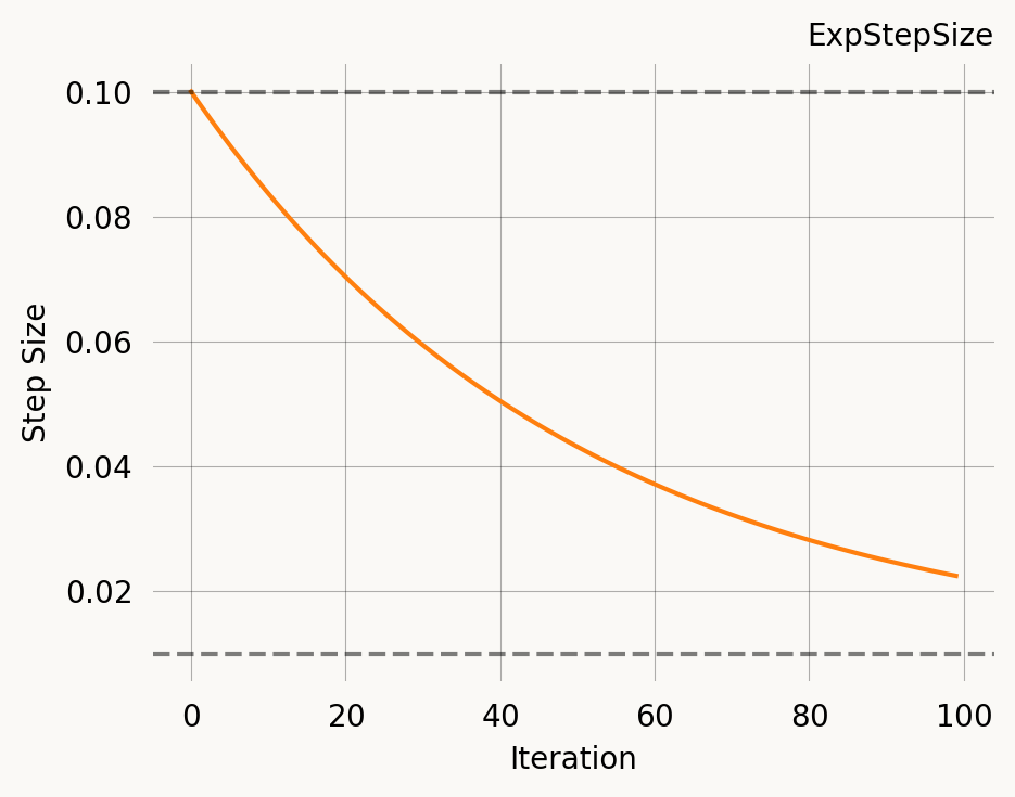
%%monitor
svgd = joint_prob_graph.svgd(
observed_data=observations,
fixed=[(2, mutation_rate)],
n_iterations=100,
n_particles=200,
prior=[
GaussPrior(ci=[5, 25]),
GaussPrior(ci=[0, 3]),
None
],
learning_rate=ExpStepSize(first_step=0.1, last_step=0.01, tau=50.0),
)
svgd.summary()Parameter Fixed MAP Mean SD HPD 95% lo HPD 95% hi
0 No 10.7539 13.0774 3.9253 6.9923 21.3284
1 No 1.1761 1.3453 0.5162 0.4344 2.4245
2 Yes 1.0000 NA NA NA NA
Particles: 200, Iterations: 100svgd.plot_ci(ci_method='hpd')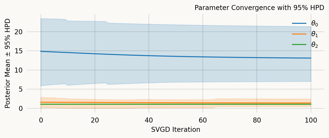
svgd.plot_convergence() ;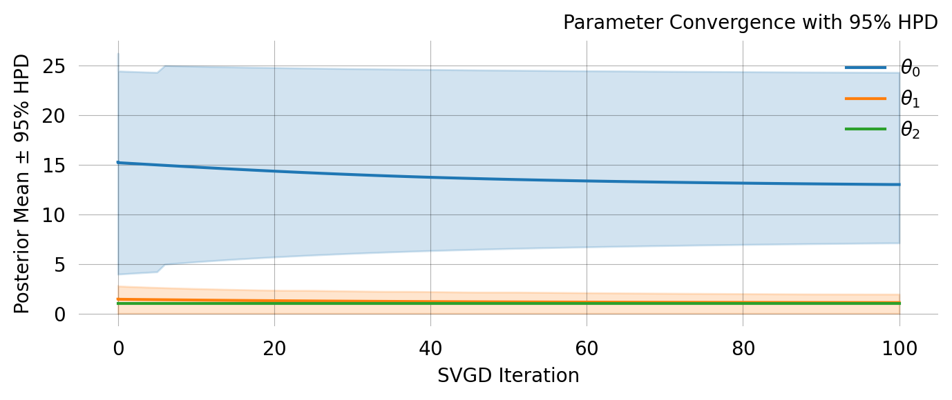
svgd.plot_trace()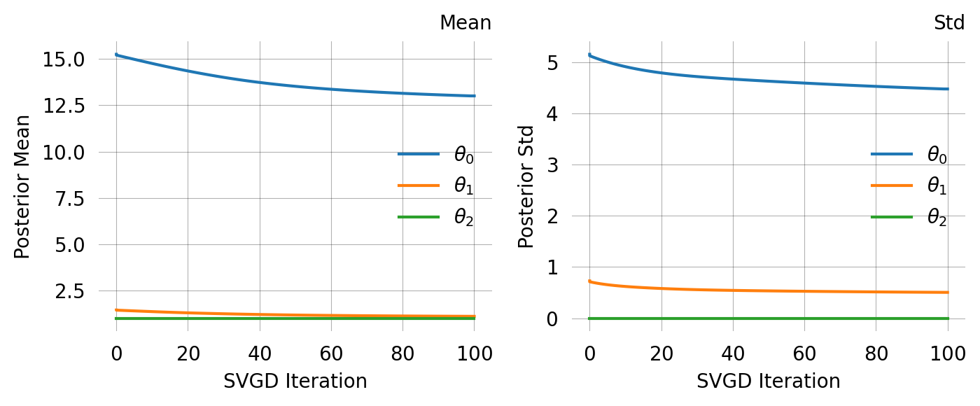
svgd.map_estimate_from_particles()([10.753870631037818, 1.1760808977707924, 1.0], -1473.625666296518)svgd.plot_hdr()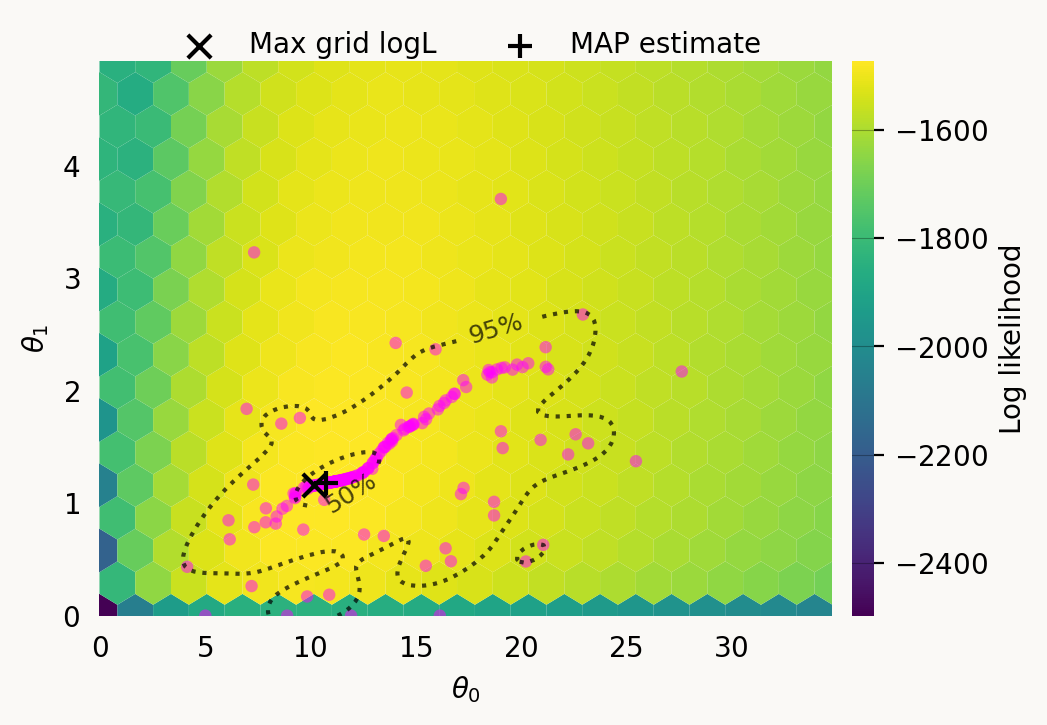
svgd.plot_hdr(hexgrid=False) ;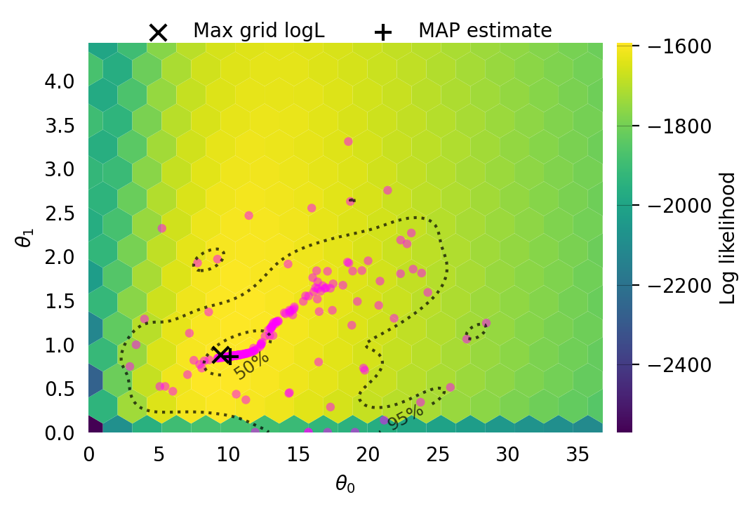
svgd.plot_pairwise(true_theta=true_theta) ;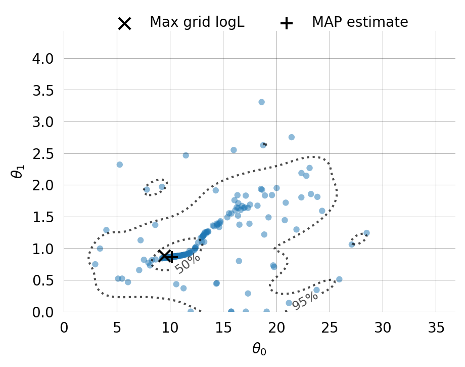
svgd.animate_pairwise(true_theta=true_theta)Example data
Simulation of two-island model:
NB: Simulation requires the msprime and tskit packages, both available as conda packages.
import msprime
import pandas as pd
import numpy as np
import matplotlib.pyplot as plt
%config InlineBackend.figure_format = 'retina'
def derived_counts(ts, rec_rate):
records = []
for var in ts.variants():
p, g = var.site.position, var.genotypes
records.append((int(p), p*rec_rate, g.sum()))
df = pd.DataFrame().from_records(
records, columns=["pos", "gen_pos", "count"]
)
return df
mut_rate = 5e-10
rec_rate = 1e-8
nr_samples = 5
seq_length = 100_000_000
pop1_size, pop2_size, anc_pop_size = 20_000, 10_000, 15_000
migr_pop1_to_pop2 = 1e-4
migr_pop2_to_pop1 = 5e-4
demography = msprime.Demography()
demography.add_population(name="pop1", initial_size=pop1_size)
demography.add_population(name="pop2", initial_size=pop2_size)
demography.set_migration_rate(source="pop1", dest="pop2", rate=migr_pop1_to_pop2)
demography.set_migration_rate(source="pop2", dest="pop1", rate=migr_pop2_to_pop1)
ts = msprime.sim_ancestry(samples={"pop1": nr_samples, "pop2": 0}, ploidy=1,
demography=demography, recombination_rate=rec_rate,
sequence_length=seq_length, random_seed=12)
ts = msprime.sim_mutations(ts, rate=mut_rate, random_seed=5678)
df = derived_counts(ts, rec_rate)
df.to_csv("island_model_derived_counts.csv", index=False)# # isolation with migration (IM) model:
# demography = msprime.Demography()
# demography.add_population(name="pop1", initial_size=pop1_size)
# demography.add_population(name="pop2", initial_size=pop2_size)
# demography.set_migration_rate(source="pop1", dest="pop2", rate=migr_pop1_to_pop2)
# demography.set_migration_rate(source="pop2", dest="pop1", rate=migr_pop2_to_pop1)
# demography.add_population(name="ancestral", initial_size=anc_pop_size)
# demography.add_population_split(time=1000, derived=["pop1", "pop2"], ancestral="ancestral")
# ts = msprime.sim_ancestry(samples={"pop1": nr_samples, "pop2": 0}, ploidy=1,
# demography=demography, recombination_rate=rec_rate,
# sequence_length=seq_length, random_seed=12)
# ts = msprime.sim_mutations(ts, rate=mut_rate, random_seed=5678)
# df = derived_counts(ts, rec_rate)
# df.to_csv("IM_model_derived_counts.csv", index=False)Get pairs of variants in the specified distance range.
def pairs_in_range(nums, diff_lo, diff_hi):
n = len(nums)
lo, hi = 1, 1
pairs = []
for i in range(n):
if lo <= i:
lo = i + 1
while lo < n and nums[lo] - nums[i] < diff_lo:
lo += 1
if hi <= i:
hi = i + 1
while hi < n and nums[hi] - nums[i] <= diff_hi:
hi += 1
for j in range(lo, hi):
pairs.append((i, j))
return pairs
df = pd.read_csv("island_model_derived_counts.csv")
col = "pos" # can also use "gen_pos"
distance, tolerance = 5000, 500
min_dist, max_dist = distance - tolerance, distance + tolerance
records = []
for i, j in pairs_in_range(df[col].values, min_dist, max_dist):
records.append((df.at[i, col], df.at[j, col], df.at[i, "count"], df.at[j, "count"]))
pairs = pd.DataFrame.from_records(records, columns=["pos1", "pos2", "count1", "count2"])
pairs.head()| pos1 | pos2 | count1 | count2 | |
|---|---|---|---|---|
| 0 | 160020 | 164783 | 1 | 3 |
| 1 | 307248 | 311878 | 4 | 1 |
| 2 | 516495 | 521242 | 2 | 1 |
| 3 | 948820 | 953791 | 1 | 3 |
| 4 | 1784175 | 1788903 | 1 | 1 |
We allow multiple SNPs from the same tree, but each SNP can only be part of a single pair. Remove pairs that share a position with another pair:
mask = (pairs.pos1 == pairs.pos1.shift()) | (pairs.pos2 == pairs.pos2.shift())
filtered_pairs = pairs.loc[~mask, :]
filtered_pairs.head()| pos1 | pos2 | count1 | count2 | |
|---|---|---|---|---|
| 0 | 160020 | 164783 | 1 | 3 |
| 1 | 307248 | 311878 | 4 | 1 |
| 2 | 516495 | 521242 | 2 | 1 |
| 3 | 948820 | 953791 | 1 | 3 |
| 4 | 1784175 | 1788903 | 1 | 1 |
Plot position differences for pairs of variants:
plt.hist(filtered_pairs.pos2 - filtered_pairs.pos1, bins=10) ;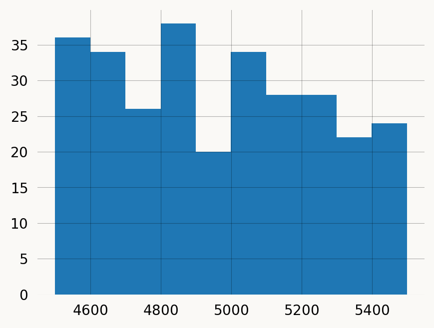
n = len(filtered_pairs)
observations = np.zeros((n, nr_samples), dtype=int)
observations
for i, pair in enumerate(filtered_pairs[["count1", "count2"]].values):
observations[i, pair] = 1msg = f"""
Two-locus observations across {nr_samples} samples of {seq_length/1e6:.0f} Mb:
Mutation rate:
{mut_rate} events/site/generation
Recombination rate:
{rec_rate} crossovers/base/generation
Haploid population sizes:
pop1: {pop1_size}
pop2: {pop2_size}
Migration rate:
pop1 -> pop2: {migr_pop1_to_pop2}
pop2 -> pop1: {migr_pop2_to_pop1}
"""
print(msg)
Two-locus observations across 5 samples of 100 Mb:
Mutation rate:
5e-10 events/site/generation
Recombination rate:
1e-08 crossovers/base/generation
Haploid population sizes:
pop1: 20000
pop2: 10000
Migration rate:
pop1 -> pop2: 0.0001
pop2 -> pop1: 0.0005
Can you make a model and find the true parameters?