Bayesian Inference with SVGD (Stein Variational Gradient Descent)
To estimate model parameters and their confidence intervals, Phasic used uses Stein Variational Gradient Descent (SVGD), which represents the posterior with a set of particles (parameter vectors) and combines ideas from optimization, kernel methods, and functional analysis in a deterministic algorithm that updates these particles iteratively to move them toward the posterior distribution. SVGD exploits the PDF for gradient computation and moments for regularization. It begins with an initial set of particles (typically drawn from the prior or from a simple distribution) and iteratively transport these particles toward the posterior using gradient information. Each particle interacts with all other particles through a kernel function, with the interaction strength depending on the distance between particles. This interaction ensures that particles spread out to cover the posterior distribution, allowing extraction of not only the most likely parameter value (MAP estimate) but also a confidence interval of the estimate.
Such inference is not possible in the standard matrix formulation of phase-type distributions where the large number of likelihood computations required would each be O(n^3). In Phasic, the algorithm of the gaussian elimination on the graph fully exploits the sparseness of state spaces bringing the complexity closer to n^2. Because Phasic records and caches the elimination trace, this computation is only done once, removing a dimension of complexity for all subsequent likelihood evaluations. For an expose of these tricks and innovations see Math and Algorithms, Architecture, Caching and Sharing.
:::
from phasic import ( Graph, with_ipv, GaussPrior, HalfCauchyPrior, DataPrior, Adam, ExpStepSize, ExpRegularization, clear_caches, set_log_level) # ALWAYS import phasic first to set jax backend correctlyimport numpy as npimport jax.numpy as jnpimport pandas as pdfrom typing import Optionalimport matplotlib.pyplot as pltfrom matplotlib.colors import LogNormimport seaborn as sns%config InlineBackend.figure_format ='svg'from tqdm.auto import tqdmfrom vscodenb import set_vscode_themeset_log_level('INFO')np.random.seed(42)set_vscode_theme()sns.set_palette('tab10')clear_caches()
Lets make a coalescent moddel with one parameter, the coalescent rate:
nr_samples =4@with_ipv([nr_samples]+[0]*(nr_samples-1))def coalescent_1param(state): transitions = []for i inrange(state.size):for j inrange(i, state.size): same =int(i == j)if same and state[i] <2:continueifnot same and (state[i] <1or state[j] <1):continue new = state.copy() new[i] -=1 new[j] -=1 new[i+j+1] +=1 transitions.append([new, [state[i]*(state[j]-same)/(1+same)]])return transitions
Construct the graph and set some value of the model parameter:
graph = Graph(coalescent_1param)graph.plot()
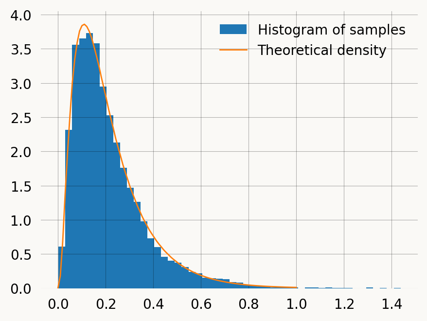
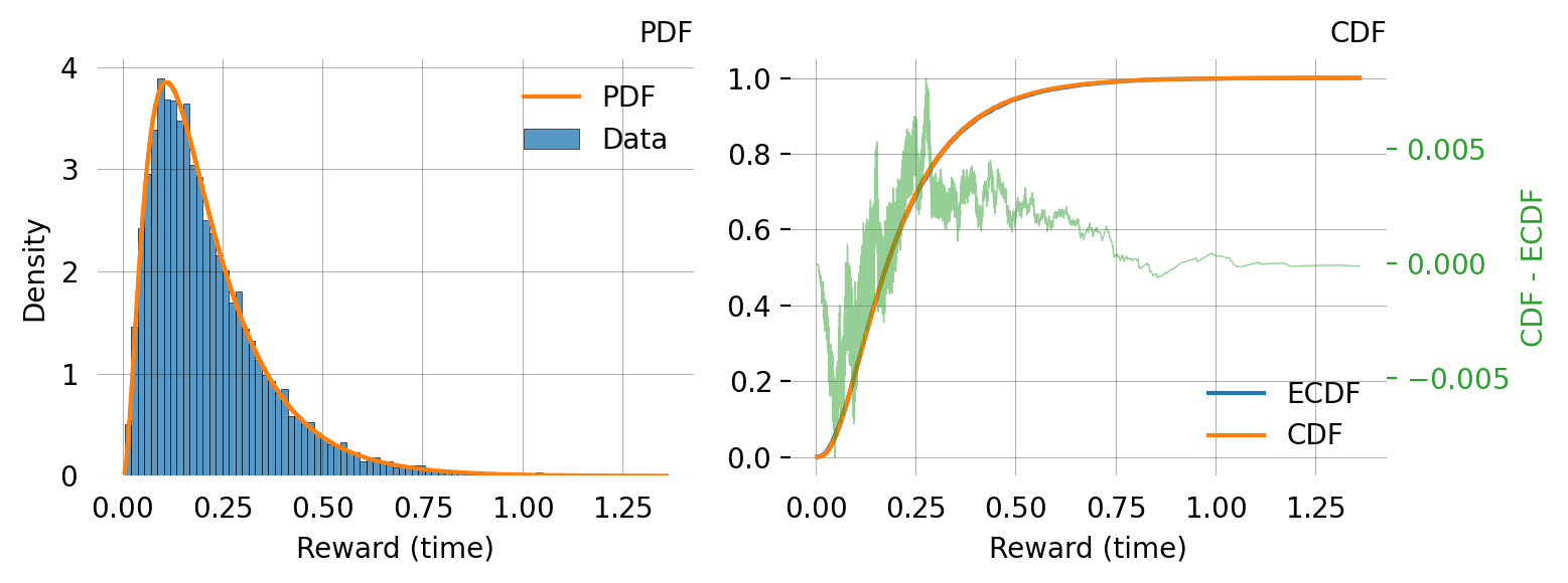
With a large set of observed times to the most recent common ancestor (TMRCA), we can fit our model to find the most likely value of the model parameter. For this turorial we will just set the model parameter to 7 and then sample from the model to get such a data set. This has the advantage that we know what the model parameter is supposed to be.
Parameter  Fixed      MAP        Mean       SD         HPD 95% lo   HPD 95% hi
0          No         7.0421     6.9476     0.1643     6.7700       7.3169

Particles: 24, Iterations: 200
svgd.learning_rate
0.0001
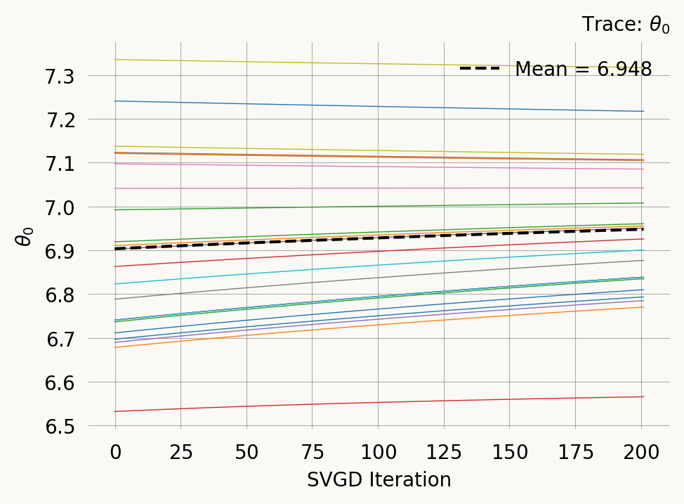
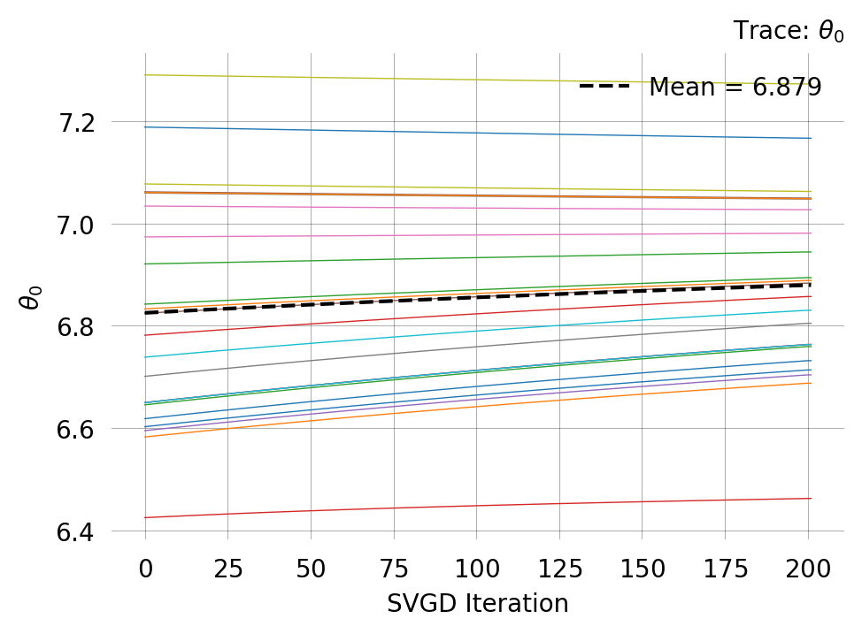
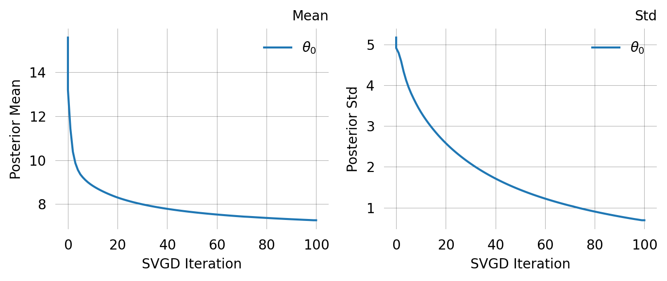
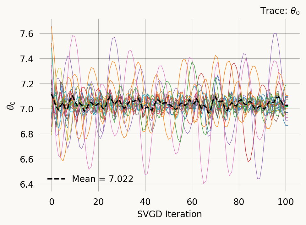
However, you should always evaluate convergence of the SVGD optimization. The plot_trace, shows the parameter values of each particle across iterations:
svgd.plot_trace();
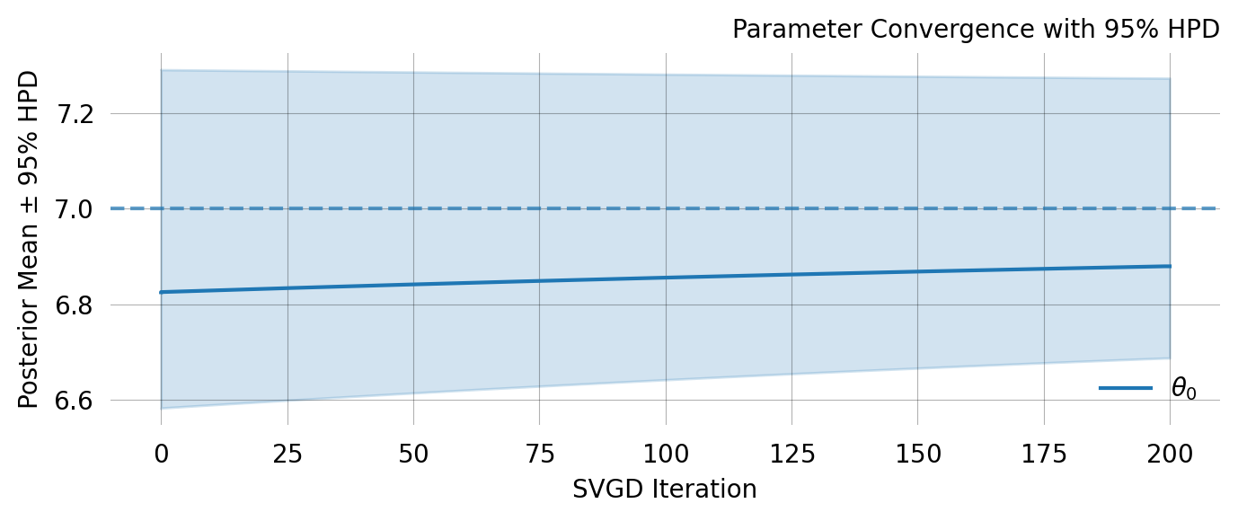
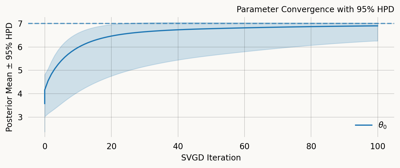
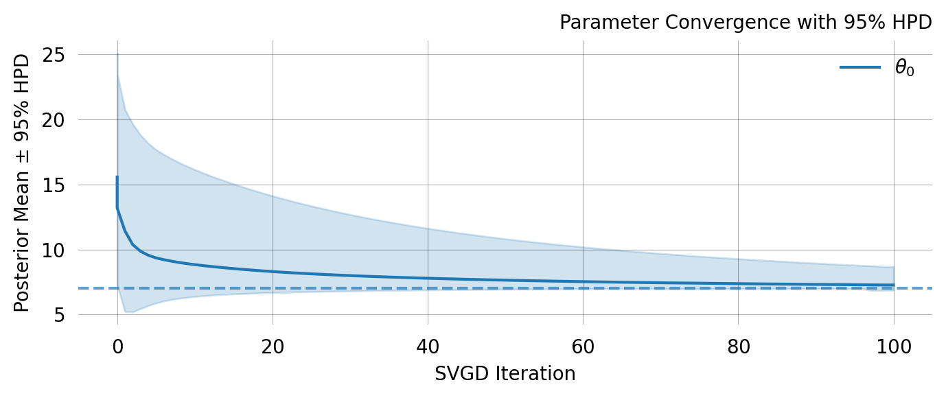
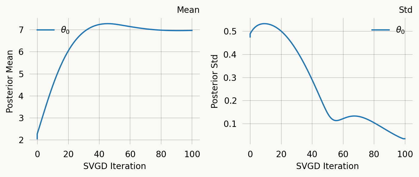
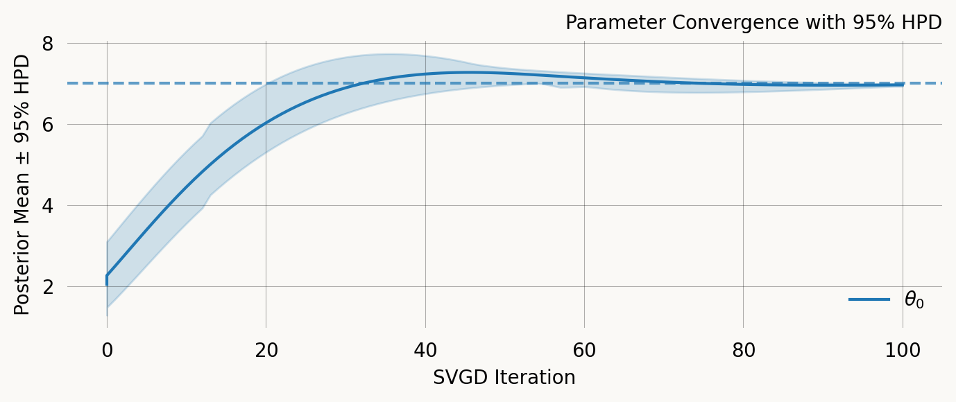
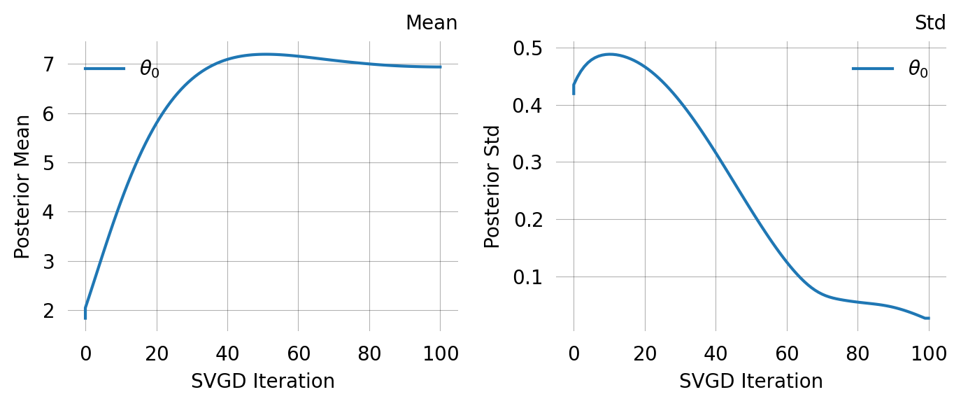
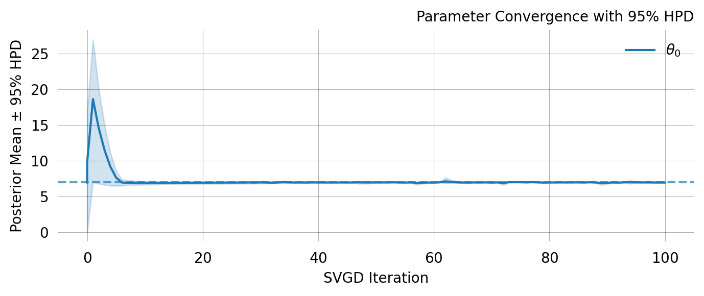
The distribution of particle values describe the posterior distribution from which a mean and CI can be computed:
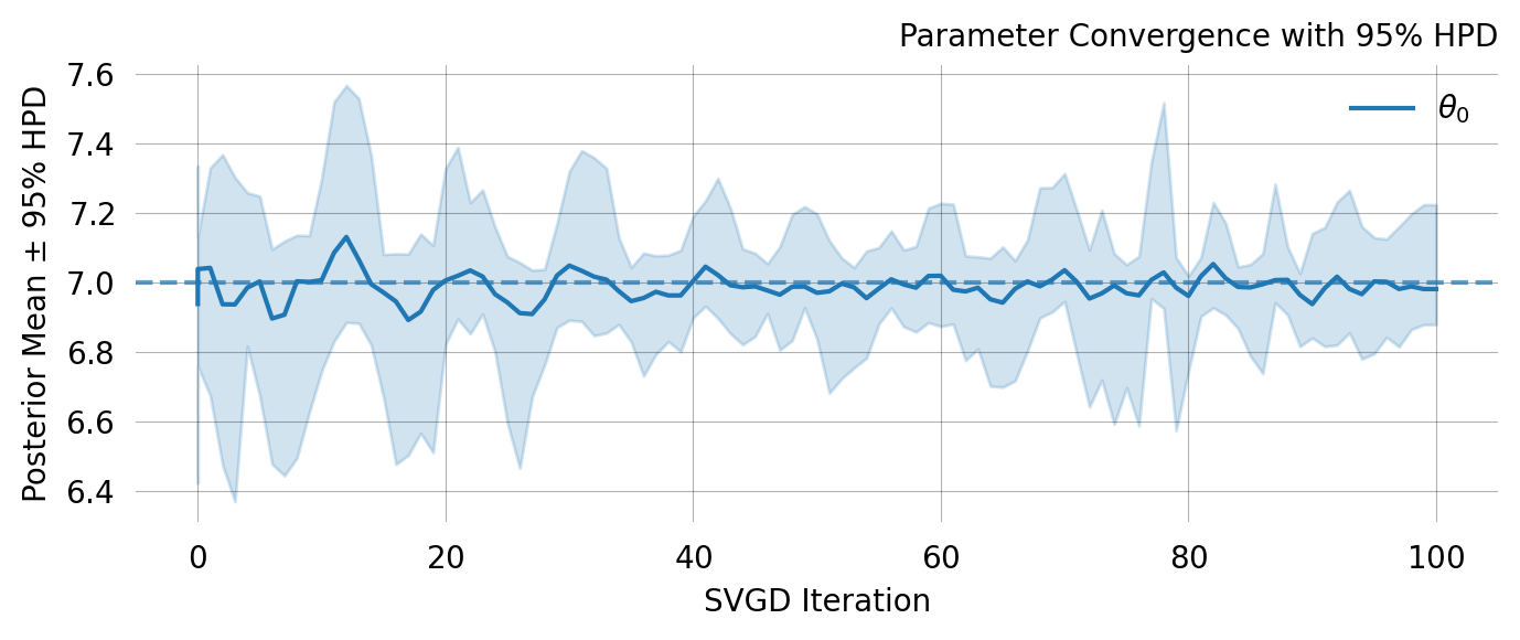
svgd.plot_ci(true_theta=true_theta) ;
A nice property of SVGD is that you can easily evaluate if the optimization converges. In this case it clearly does not. Fortunately there are several easy remedies for this as shown below.
Prior
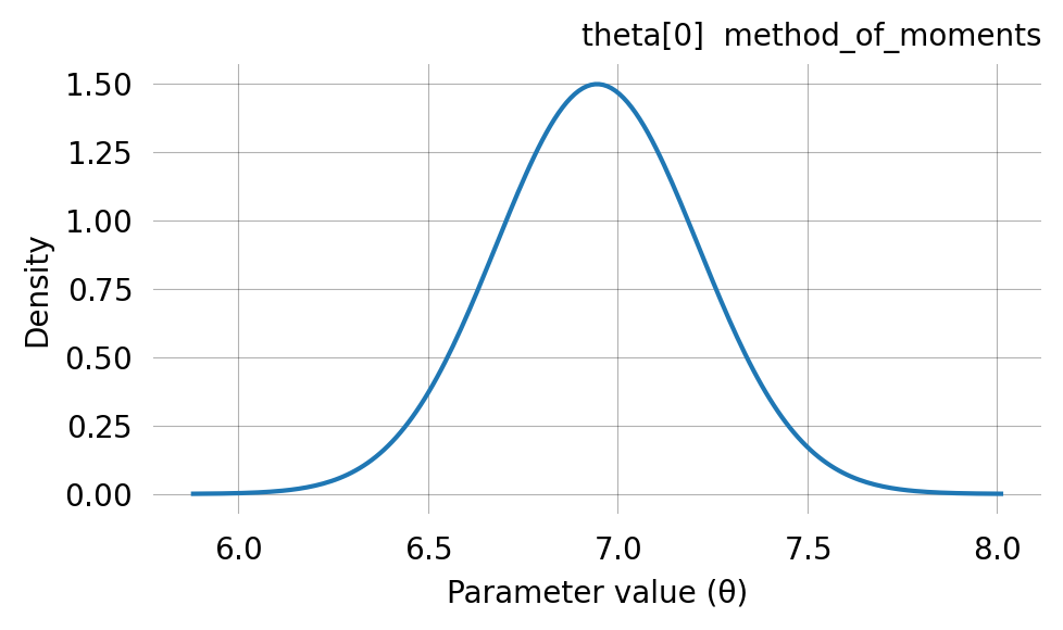
The prior distribution used in Bayesian inference represents our prior belief, I.e. our knowledge about what range of values the parameter can reasonably take. Phasic comes with two types of priors that are easily defined from basic knowledge about the parameter. The default behaviour of Phasic is to use a Gaussian prior centered on a rough estimate of each parameter using method-of-moments. To see the prior used, you can can plot it like this:
svgd.prior.plot() ;
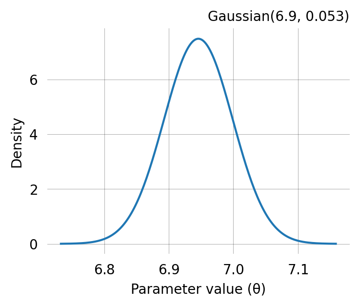
or reconstruct the GaussPrior from its properties:
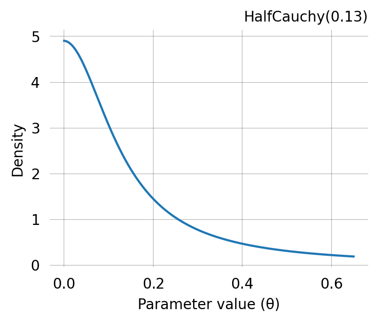
The GaussPrior and HalfCauchyPrior classes provide the log-probabilities needed for SVGD. If you want to provide your own prior function, it must return such log-probabilities.
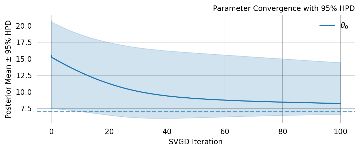
Lets add the prior to SVGD inference and rerun it.
NOT CONVERGED after 102 iterations
Detected Issues:
⚠ Did not converge within n_iterations
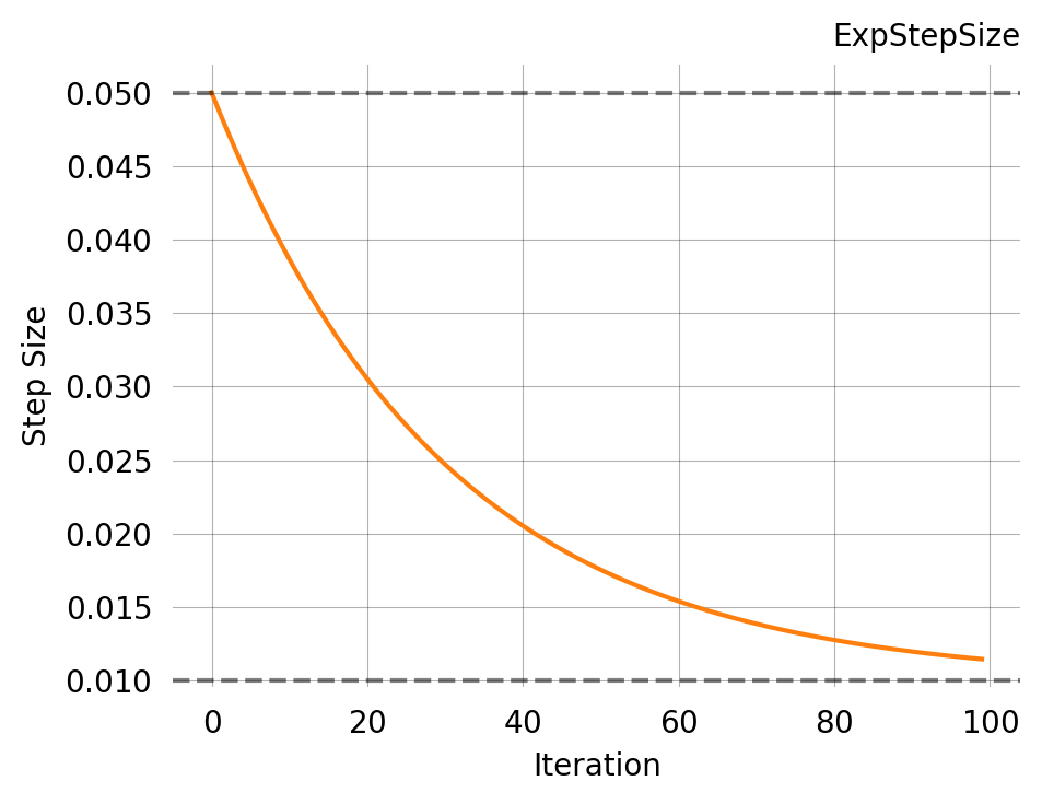
Learning Rate: Not converged - use decay schedule for better convergence
ExpStepSize(
first_step=0.00015000000000000001,
last_step=1e-05,
tau=51.0
)
Particles: High ESS ratio (1.00) - could reduce particles
n_particles=20
Iterations: Did not converge
Increase to n_iterations=153
Optimizer: Consider using an adaptive optimizer
Options (from phasic import Adam, SGDMomentum, RMSprop, Adagrad):
Adam(lr=0.01) - Adaptive LR + momentum (recommended)
SGDMomentum(lr=0.01) - Momentum only
RMSprop(lr=0.001) - Adaptive LR, no momentum
Adagrad(lr=0.01) - Cumulative gradient scaling
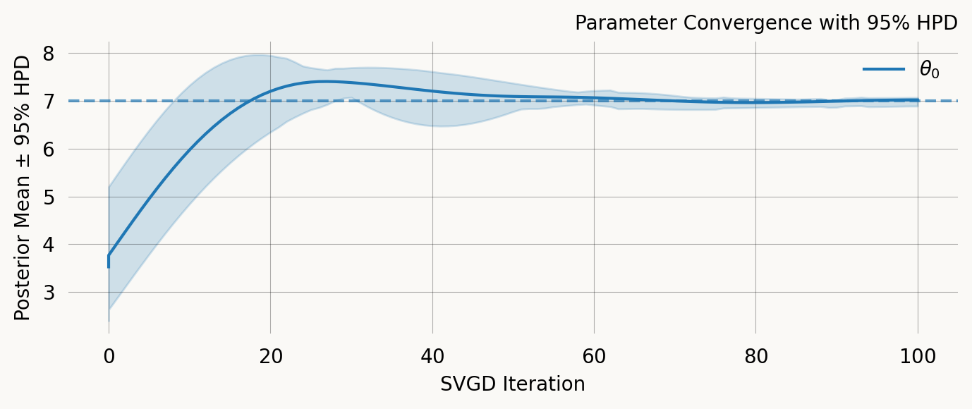
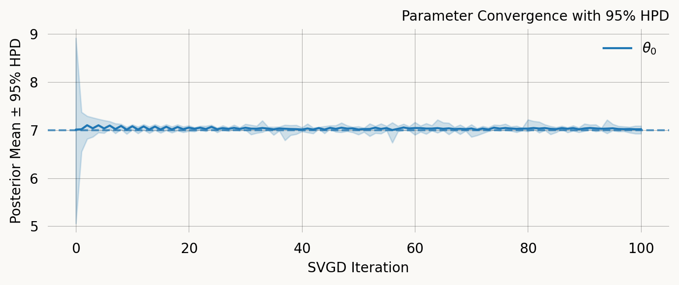
That is better, but it still does not converge to the true theta value. We can change the learning rate from its default value of 0.01:
Phasic provides three optimizers for SVGD that offer adaptive per-parameter learning rates. These can be particularly useful when gradients have vastly different scales across parameters or when fixed step sizes cause oscillation.
Adam
When using Adam, the learning_rate parameter passed to SVGD is ignored in favor of the optimizer’s learning rate.
Adam (Adaptive Moment Estimation) maintains running estimates of two quantities for each parameter:
First moment (m): An exponentially weighted average of past gradients (momentum)
Second moment (v): An exponentially weighted average of past squared gradients (gradient variance)
Update rule:
\begin{align}
m &\leftarrow \beta_1 \cdot m + (1 - \beta_1) \cdot g \\
v &\leftarrow \beta_2 \cdot v + (1 - \beta_2) \cdot g^2 \\[0.5em]
\hat{m} &= \frac{m}{1 - \beta_1^t} \\[0.5em]
\hat{v} &= \frac{v}{1 - \beta_2^t} \\[0.5em]
\theta &\leftarrow \theta - \alpha \cdot \frac{\hat{m}}{\sqrt{\hat{v}} + \epsilon}
\end{align}
Each parameter gets its own effective learning rate:
Parameters with consistently large gradients \rightarrow larger \hat{v}\rightarrow smaller effective step
Parameters with consistently small gradients \rightarrow smaller \hat{v}\rightarrow larger effective step
This automatic scaling helps when different parameters naturally have different gradient magnitudes.
When fixed learning rate works well:
Well-behaved optimization landscapes
Parameters with similar gradient scales
When you’ve tuned the learning rate carefully
When Adam helps:
Large datasets causing large gradient magnitudes
Parameters with vastly different scales
“Shark teeth” oscillation patterns in convergence
When you want reasonable results without extensive tuning
Tuning Guidelines:
learning_rate: Start with 0.001-0.01. If convergence is too slow, increase. If unstable, decrease.
beta1: 0.9 works well for most cases. Lower values (0.8) give less momentum.
beta2: 0.999 is standard. Lower values (0.99) adapt faster to gradient changes.
epsilon: Rarely needs adjustment. Increase to 1e-7 if you see numerical issues.
Consider Adam when you observe:
Oscillating convergence (“shark teeth” pattern in loss)
Different parameters converging at different rates
Sensitivity to learning rate choice
Large datasets** causing large gradient magnitudes
Stick with fixed learning rate when:
Convergence is already smooth and fast
You’ve tuned the learning rate well for your problem
You want minimal computational overhead
The optimization landscape is well-behaved
Kingma and Ba (2014) - Adam: A Method for Stochastic Optimization. arXiv:1412.6980.
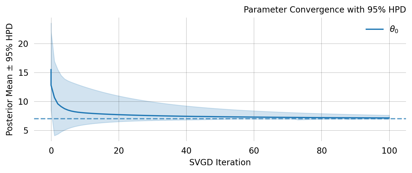
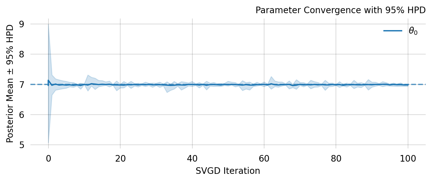
from phasic import Adamoptimizer = Adam( learning_rate=0.001, # Base learning rate, scaled per-parameter by Adam (alpha) beta1=0.9, # Decay rate for first moment (momentum). Higher = more smoothing beta2=0.999, # Decay rate for second moment. Higher = longer memory of gradient magnitudes epsilon=1e-8# Small constant to prevent division by zero)
Parameter  Fixed      MAP        Mean       SD         HPD 95% lo   HPD 95% hi
0          No         6.9885     6.9610     0.0342     6.9243       6.9885

Particles: 24, Iterations: 100
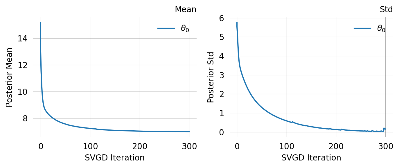
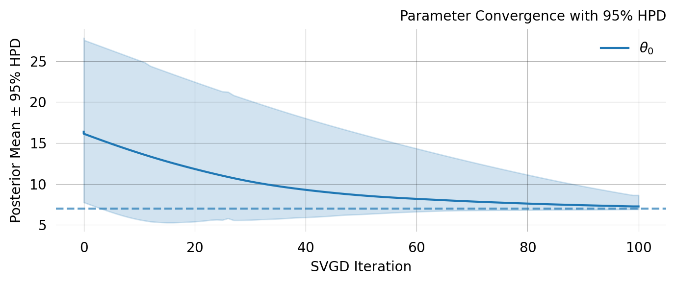
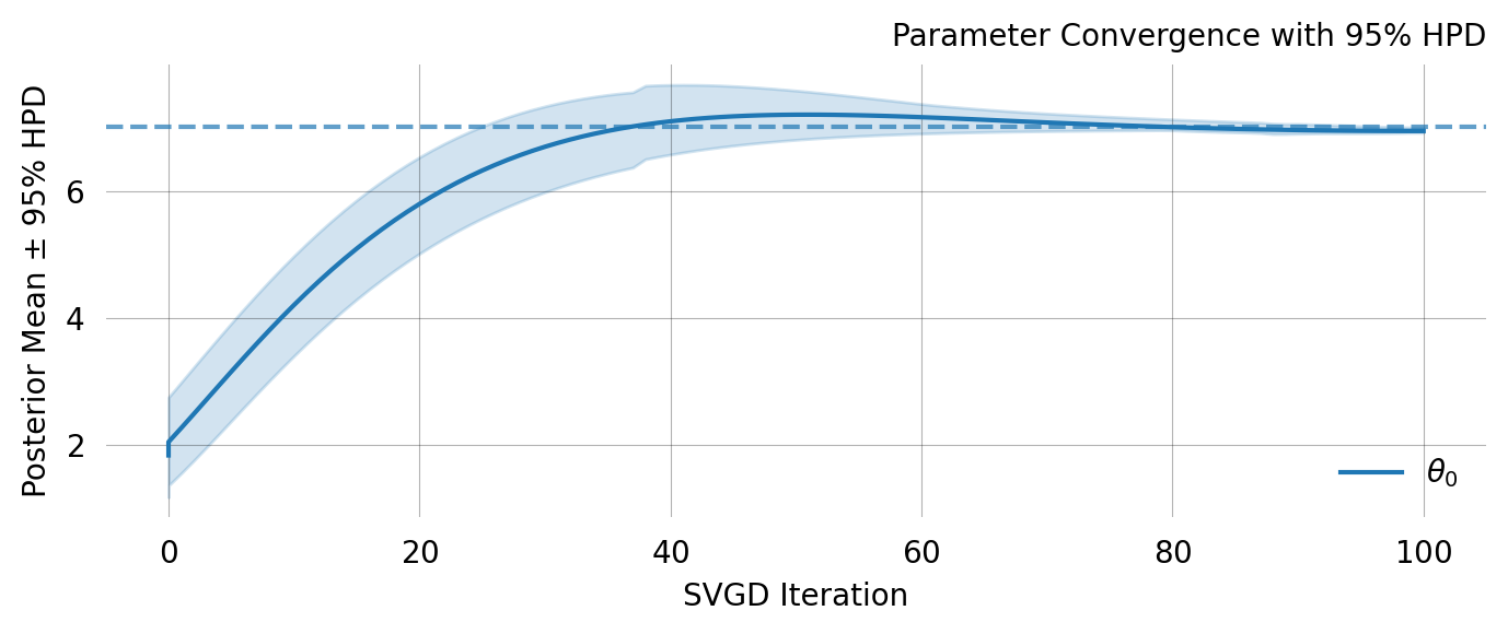
svgd.plot_convergence() ;
svgd.plot_ci(true_theta=true_theta) ;
svgd.plot_trace() ;
SGDMomentum
SGDMomentum (SGD with momentum) accumulates velocity in directions of persistent gradient descent, helping accelerate convergence and dampen oscillations. Update rule:
\begin{align}
v &= m * v + g \\
\theta &= \theta + (l * v)
\end{align}
where g is gradient l is learning rate, and m and v are the first and second moments.
Parameter  Fixed      MAP        Mean       SD         HPD 95% lo   HPD 95% hi
0          No         7.0319     7.0224     0.0689     6.8649       7.1038

Particles: 24, Iterations: 100
svgd.plot_convergence() ;
svgd.plot_ci(true_theta=true_theta) ;
svgd.plot_trace() ;
RMSprop
RMSprop(Hinton 2012) divides the learning rate by an exponentially decaying average of squared gradients, adapting per-parameter. Update rule:
$$ \begin{align}
v &= d * v + (1 - d) * g^2 \\
\theta &= \theta + \frac{l * g}{\sqrt{v} + \epsilon}
\end{align} $$
where g is gradient l is learning rate, d is the decay and v is
from phasic.svgd import RMSpropoptimizer = RMSprop( learning_rate=1, # Base learning rate (default 0.001) decay=0.99, # Decay rate for squared gradient average epsilon=1e-8# Numerical stability)svgd = graph.svgd( observed_data, optimizer=optimizer,)svgd.summary()
Parameter  Fixed      MAP        Mean       SD         HPD 95% lo   HPD 95% hi
0          No         7.0352     6.8296     0.3088     6.1385       7.0360

Particles: 24, Iterations: 100
svgd.plot_convergence() ;
svgd.plot_ci(true_theta=true_theta) ;
svgd.plot_trace() ;
Adagrad
Adagrad(Duchi et al. 2011) accumulates the sum of squared gradients, giving smaller learning rates to parameters with large accumulated gradients. Update rule: