Joint probability

Phase-type distributions can be extended to model joint probabilities of multiple random variables. This is particularly important in applications like population genetics, where we might be interested in the joint distribution of coalescence times for multiple lineages, or in reliability theory, where we might want the joint distribution of failure times for multiple components. This section shows how to compute exact joint probabilities.

from phasic import (Graph, with_ipv, # ALWAYS import phasic first to set jax backend correctly
    StateIndexer, Property
)
import sys
import numpy as np
import pandas as pd
import matplotlib.pyplot as plt
from matplotlib.colors import LogNorm
import seaborn as sns
%config InlineBackend.figure_format = 'svg'
from typing import Optional
from tqdm.auto import tqdm
from functools import partial
from vscodenb import set_vscode_theme, vscode_theme
from itertools import combinations, combinations_with_replacement
all_pairs = partial(combinations_with_replacement, r=2)

np.random.seed(42)
set_vscode_theme()
sns.set_palette('tab10')

nr_samples = 4
indexer = StateIndexer(
    lineage=[
        Property('descendants', min_value=1, max_value=nr_samples),
    ]
)

@with_ipv([nr_samples]+[0]*(nr_samples-1))
def coalescent(state):
    transitions = []
    for i, j in all_pairs(indexer.lineage):
        p1 = indexer.lineage.index_to_props(i)
        p2 = indexer.lineage.index_to_props(j)
        same = int(i == j)
        if same and state[i] < 2:
            continue
        if not same and (state[i] < 1 or state[j] < 1):
            continue 
        new = state.copy()
        new[i] -= 1
        new[j] -= 1
        descendants = p1.descendants + p2.descendants
        k = indexer.lineage.props_to_index(descendants=descendants)
        new[k] += 1
        transitions.append([new, state[i]*(state[j]-same)/(1+same)])
    return transitions

Now lets construct the joint probability graph. In addition to a mutation rate, you must specify an upper bound on the number of discrete rewards you want to account for. You can specify a maximum discrete value of each feature (how many tons of each kind you want to account for) using the reward_limit keyword argument. This takes both a scalar argument for a maximum applied to all features or an array with a maximum for each feature. You can also use the tot_reward_limit keyword argument to specify a maximum on total rewards for each feature combination. Both arguments may be specified to define the upper bound.

Since we only model a subset of feature combinations, the joint distribution is deficient. The deficit is the total probability of feature combinations beyond the upper bound. You can easily compute this as one minus the sum of joint probabilities.

graph = Graph(coalescent)
graph.plot()

mutation_rate = 0.1
joint_prob_graph = graph.joint_prob_graph(indexer, tot_reward_limit=2, mutation_rate=mutation_rate)
joint_prob_graph.vertices_length()

joint_prob_graph.plot(nodesep=0.3)

Compute the joint probabilities:

joint_prob_table = joint_prob_graph.joint_prob_table()
joint_prob_table

	descendants_1	descendants_2	descendants_3	descendants_4	prob
t_vertex_index
9	0	0	0	0	0.710227
18	0	1	0	0	0.060979
20	1	0	0	0	0.126890
23	0	0	1	0	0.039457
30	0	2	0	0	0.007658
31	2	0	0	0	0.014744
32	1	0	1	0	0.010394
33	0	0	2	0	0.002989
34	1	1	0	0	0.009097
35	0	1	1	0	0.001087

Deficit:

(1 - joint_prob_table['prob'].sum()).item()

0.016476095092311294

ton_pair = ['descendants_2', 'descendants_3']
plot_df = joint_prob_table[ton_pair + ['prob']].groupby(ton_pair).sum().reset_index()   
plot_df = plot_df.pivot(index=ton_pair[1], columns=ton_pair[0], values='prob')

with vscode_theme(style='ticks'):
    ax = sns.heatmap(
        plot_df,
        cmap='viridis',
        cbar_kws={'label': 'Probability'},
        xticklabels=1,
        yticklabels=1,
        norm=LogNorm(),
    )
    ax.set(xlabel=ton_pair[0], ylabel=ton_pair[1])
    ax.invert_yaxis()
plt.show()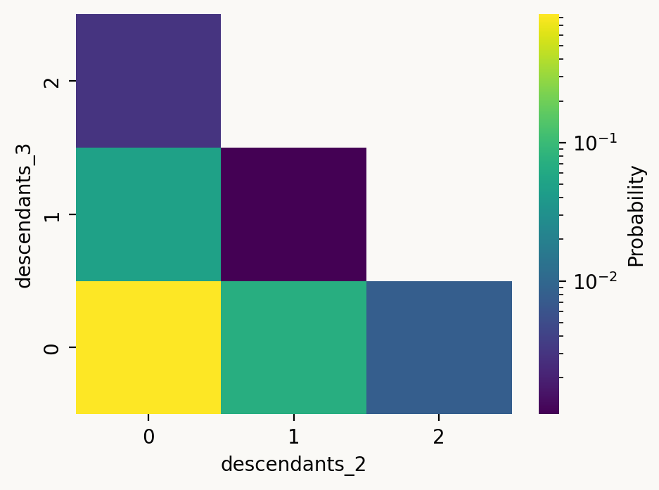

Note that the joint probability graph does not have meaningful moments and pdf. E.g., the expectation is inf because of the infinite loop between the trash states:

joint_prob_graph.expectation()

inf

The joint probabilities are extracted as the sojourn times of appropriate transient states connecting only to the absorbing state:

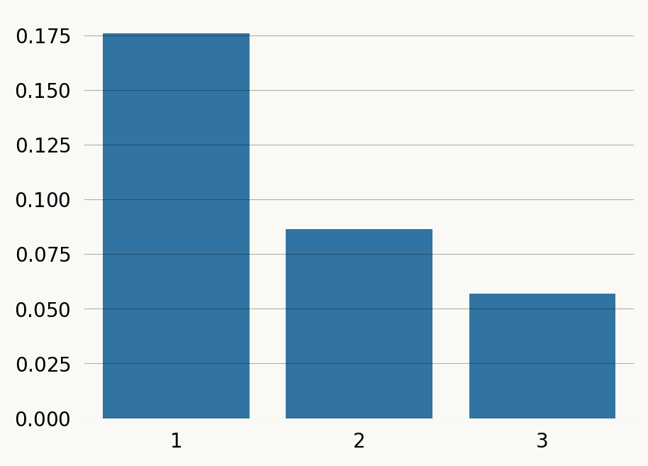
tons = np.arange(1, nr_samples)
marginals = [np.sum(joint_prob_table[f'descendants_{t}'] * joint_prob_table['prob']) for t in tons]
sns.barplot(x=tons, y=marginals);
plt.show()