Moments and distributions

Download notebook

from phasic import Graph, with_ipv # ALWAYS import phasic first to set jax backend correctly
import sys
import numpy as np
import pandas as pd
import matplotlib.pyplot as plt
from matplotlib.colors import LogNorm
import seaborn as sns
from vscodenb import set_vscode_theme

np.random.seed(42)
set_vscode_theme()
sns.set_palette('tab10')

Overriding theme from NOTEBOOK_THEME environment variable. <phasic._DeviceListFilter object at 0x17c6e4f90>

Construct a graph:

nr_samples = 4

@with_ipv([nr_samples]+[0]*(nr_samples-1))
def coalescent(state):
    transitions = []
    for i in range(state.size):
        for j in range(i, state.size):            
            same = int(i == j)
            if same and state[i] < 2:
                continue
            if not same and (state[i] < 1 or state[j] < 1):
                continue 
            new = state.copy()
            new[i] -= 1
            new[j] -= 1
            new[i+j+1] += 1
            transitions.append((new, state[i]*(state[j]-same)/(1+same)))
    return transitions

graph = Graph(coalescent)
graph.plot()

Overriding theme from NOTEBOOK_THEME environment variable. <phasic._DeviceListFilter object at 0x17c6e4f90>

Show states nicely as data frame:

labels = [f"{i+1}'ton" for i in range(nr_samples)]

pd.DataFrame(graph.states(), columns=labels)

	1'ton	2'ton	3'ton	4'ton
0	0	0	0	0
1	4	0	0	0
2	2	1	0	0
3	0	2	0	0
4	1	0	1	0
5	0	0	0	1

This phase-type distribution models the time until all lineages have coalesced. For convenience, we can get its expectation and variance like this:

graph.expectation()

1.4999999999999996

graph.variance()

1.1388888888888893

But if you want you can get any number of moments like this (here three):

graph.moments(3)

[1.4999999999999996, 3.388888888888888, 10.583333333333332]

We can find the expected waiting time given that we start in any of the states, not just the starting state:

graph.expected_waiting_time()

[1.4999999999999996, 1.4999999999999996, 1.333333333333333, 1.0, 1.0, 0.0]

Expected time spent in each state (exact):

graph.expected_sojourn_time()

[0.0,
 0.16666666666666663,
 0.33333333333333326,
 0.3333333333333333,
 0.6666666666666666,
 0.0]

Expected time spent in each state after some time:

graph.accumulated_occupancy

<bound method Graph.accumulated_occupancy of <Graph (6 vertices)>>

We can get the CDF and PDF. The distribution methods reuse cached computations and recompute only if the graph changes. Compare the running times for the first and second call to the function:

time = np.arange(0, 4, 0.001)

%%time
cdf = graph.cdf(time)

CPU times: user 213 μs, sys: 22 μs, total: 235 μs
Wall time: 238 μs

%%time
cdf = graph.cdf(time)

CPU times: user 28 μs, sys: 4 μs, total: 32 μs
Wall time: 34.1 μs

Plot PDF and CDF:

fig, (ax1, ax2) = plt.subplots(1, 2, figsize=(8, 3))
ax1.plot(time, graph.pdf(time))
ax1.set_title("PDF")
ax2.plot(time, graph.cdf(time))
ax2.set_title("CDF") ;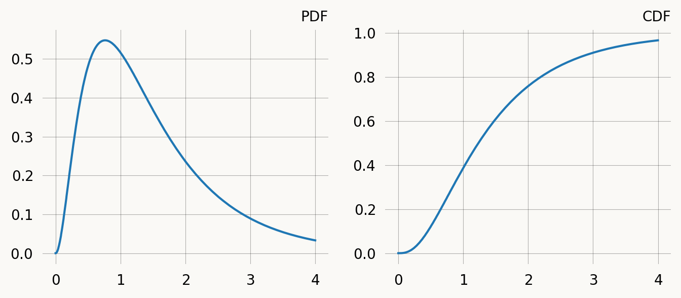

<Figure size 640x480 with 0 Axes>

Rewards

We can add rewards which are based on the number of doubletons:

graph = Graph(coalescent)
reward_matrix = graph.states().T
doubletons = reward_matrix[1]
doubletons

array([0, 0, 1, 2, 0, 0], dtype=int32)

Adding these rewards, the phase-type distribution now represent the total doubleton branch length (total length of branches with two descendants). The expectation and variance are now:

graph.expectation(doubletons), graph.variance(doubletons)

(0.9999999999999999, 2.333333333333333)

Using rewards to the moment functions etc. is much faster than changing the graph. Here is the SFS (Site Frequency Spectrum) computed in this way. The 4’ton is included to illustrate that it is represented but has expectation zero since this it the absorbing TMRCA.

labels = [f"{i+1}'ton" for i in range(reward_matrix.shape[0])]
sfs = [graph.expectation(r) for r in reward_matrix]
plt.figure(figsize=(4, 3))
sns.barplot(x=labels, y=sfs, hue=labels) ;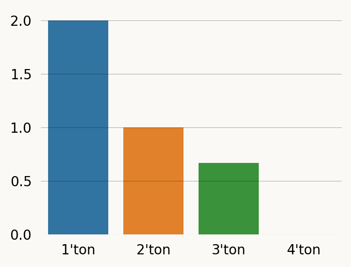

And here by doing each reward_transform:

singleton_graph = graph.reward_transform(reward_matrix[0])
singleton_graph.plot()

Overriding theme from NOTEBOOK_THEME environment variable. <phasic._DeviceListFilter object at 0x17c6e4f90>

doubleton_graph = graph.reward_transform(reward_matrix[1])
doubleton_graph.plot()

Overriding theme from NOTEBOOK_THEME environment variable. <phasic._DeviceListFilter object at 0x17c6e4f90>

tripleton_graph = graph.reward_transform(reward_matrix[2])
tripleton_graph.plot()

Overriding theme from NOTEBOOK_THEME environment variable. <phasic._DeviceListFilter object at 0x17c6e4f90>

quadrupleton_graph = graph.reward_transform(reward_matrix[3])
quadrupleton_graph.plot()

Overriding theme from NOTEBOOK_THEME environment variable. <phasic._DeviceListFilter object at 0x17c6e4f90>

sfs = [
    singleton_graph.expectation(),
    doubleton_graph.expectation(),
    tripleton_graph.expectation(),
    quadrupleton_graph.expectation()
]
plt.figure(figsize=(4, 3))
sns.barplot(x=labels, y=sfs, hue=labels) ;

Computing the (unrewarded) expectation on the reward-transforming graph produces the same result as passing the rewards to expectation, but is much slower:

graph = Graph(coalescent)
singleton_rewards = graph.states().T[0]

%%timeit
graph.expectation(singleton_rewards)

1.97 μs ± 31 ns per loop (mean ± std. dev. of 7 runs, 1,000,000 loops each)

%%timeit
graph.reward_transform(singleton_rewards).expectation()

13.1 μs ± 143 ns per loop (mean ± std. dev. of 7 runs, 100,000 loops each)

The real use of reward transformation is that it provides the full distribution of accumulated rewards. For example if we want the PDF/CDF.

graph = Graph(coalescent)
graph.plot()

Overriding theme from NOTEBOOK_THEME environment variable. <phasic._DeviceListFilter object at 0x17c6e4f90>

times = np.arange(0, 5, 0.05)
reward_matrix = graph.states().T
labels = [f"{i+1}'ton" for i in range(reward_matrix.shape[1])]

for i, rewards in enumerate(reward_matrix):
    revt_graph = graph.reward_transform(rewards)
    plt.plot(times, revt_graph.pdf(times), label=labels[i])
plt.legend() ;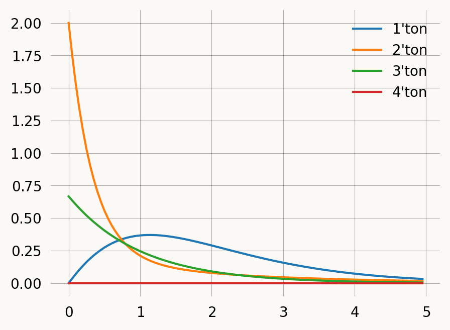

State probability and occupancy

There are also utility methods to get the state probability i.e. probabilities of occupying each state at time t.

graph = Graph(coalescent)

graph.state_probability(0.2)

[0.0,
 0.29978049956512576,
 0.4964527753776389,
 0.06299978987254216,
 0.12599957974508433,
 0.0]

We can use that to compute the expected number of lineages across time:

times = np.arange(0, 5, 0.05)
expected_lineages_left = [
    np.sum(graph.state_probability(i) 
           * np.sum(graph.states(), axis=1)) 
    for i in times
    ]

fig, ax = plt.subplots(1, 1, figsize=(4, 3))
ax.plot(times, expected_lineages_left)
ax.set_xlabel('Time')
ax.set_ylabel("Expected nr lineages") ;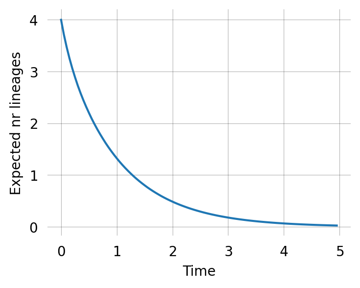

Figure 1: Expected number of lineages across time.

The same way we can also compute the expected number of each kind of lineage across time:

times = np.arange(0, 5, 0.05)
state_probs = np.array([graph.state_probability(i) * graph.states().T for i in times])
labels = [f"{i+1}'ton" for i in range(state_probs.shape[1])]
fig, axes = plt.subplots(1, 2, figsize=(6, 3))
axes[0].stackplot(times, np.sum(state_probs, axis=2).T)
axes[1].plot(times, np.sum(state_probs, axis=2), label=labels)
# plt.subplot(121).stackplot(times, np.sum(state_probs, axis=2).T)
# plt.subplot(122).plot(times, np.sum(state_probs, axis=2), label=labels)
plt.legend() ;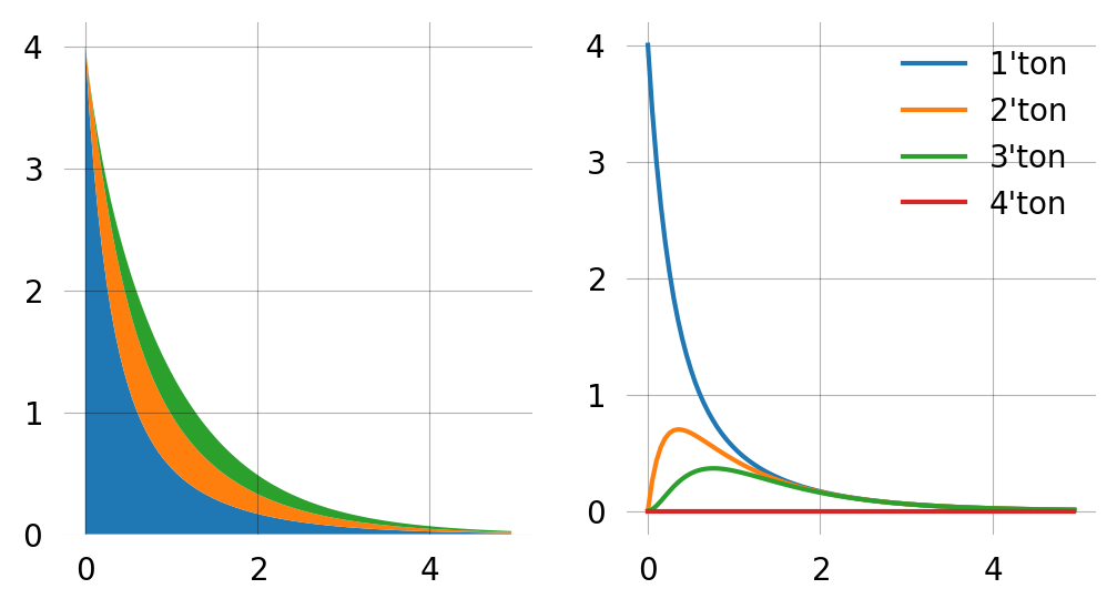

Figure 2: Expected number of lineages across time.

We can also get the accumulated visiting time of a particular state. E.g. the total doubleton branchlength before time t=1.5:

rewards = (graph.states()[:,1]>0).astype(int)
np.sum(graph.accumulated_occupancy(time=1.5) * rewards)

np.float64(0.5293813150697056)

Random sampling

The library includes functions to do random sampling. These are useful to also validate the computations

graph = Graph(coalescent)
graph.sample(5)

array([0.69917518, 0.7254702 , 0.38892427, 1.84570689, 1.35056846])

fig, ax = plt.subplots(figsize=(4, 3))
samples = graph.sample(100000)

ax.hist(samples, bins=100, density=True, label='Samples')
x = np.arange(0, 2, 0.05)

ax.plot(x, [graph.pdf(t) for t in x], label='PDF')

ax.set_xlim(0, 2)
ax.legend();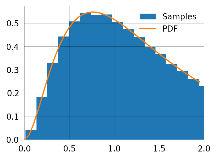

You can produce the moments from sampling if needed. This is the empirical second moment computed from samples:

np.sum(np.array(graph.sample(10000))**2).item()/10000

3.453041508940769

Compare to the exact second moment:

graph.moments(2)[1]

3.3888888888888884