Priors and schedules

This notebook provides a comprehensive reference for the prior distributions, step size schedules, and regularization schedules available in phasic for use with SVGD inference. Each class is demonstrated with its construction options, key parameters, and visual output.

from phasic import (
    Graph, with_ipv,
    # Priors
    GaussPrior, HalfCauchyPrior, DataPrior,
    # Step size schedules
    ConstantStepSize, ExpStepSize, AdaptiveStepSize, WarmupExpStepSize,
    # Regularization schedules
    ConstantRegularization, ExpRegularization, ExponentialCDFRegularization,
    # Optimizers (for examples)
    Adam,
) # ALWAYS import phasic first to set jax backend correctly
import numpy as np
import jax.numpy as jnp
import matplotlib.pyplot as plt
import seaborn as sns

np.random.seed(42)
try:
    from vscodenb import set_vscode_theme
    set_vscode_theme()
except ImportError:
    pass
sns.set_palette('tab10')

Overriding theme from NOTEBOOK_THEME environment variable. <phasic._DeviceListFilter object at 0x13a7c3e50>

Priors

GaussPrior

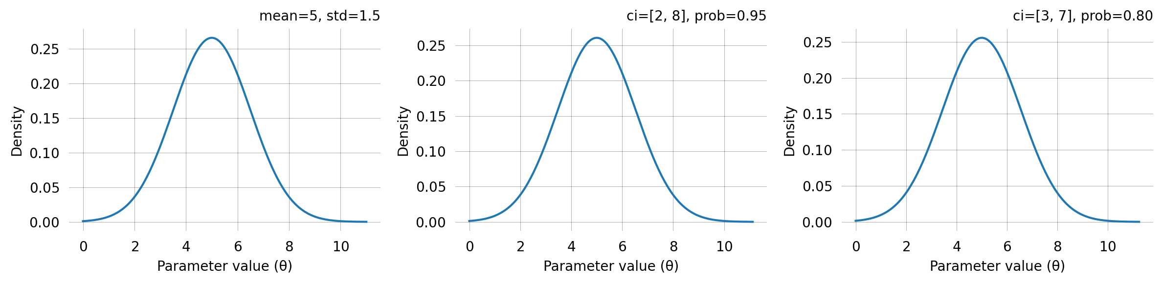
A Gaussian (normal) prior centred on a point estimate with a given spread. It can be specified in two ways:

1. Mean and standard deviation — when you know the centre and spread directly.
2. Credible interval — when you can state a range that should contain the parameter with a given probability.

The two specifications are equivalent: a 95% credible interval [low, high] maps to mean = (low + high) / 2 and std = (high - low) / (2 * z_0.975).

fig, axes = plt.subplots(1, 3, figsize=(12, 3))

# 1. Mean + std
p1 = GaussPrior(mean=5.0, std=1.5)
p1.plot(ax=axes[0], return_ax=True)
axes[0].set_title(f'mean=5, std=1.5')

# 2. 95% credible interval
p2 = GaussPrior(ci=(2.0, 8.0))
p2.plot(ax=axes[1], return_ax=True)
axes[1].set_title(f'ci=[2, 8], prob=0.95')

# 3. 80% credible interval (tighter)
p3 = GaussPrior(ci=(3.0, 7.0), prob=0.80)
p3.plot(ax=axes[2], return_ax=True)
axes[2].set_title(f'ci=[3, 7], prob=0.80')

plt.tight_layout()

<Figure size 640x480 with 0 Axes>

The credible-interval specification is often the most intuitive: “I believe the parameter is between 2 and 8 with 95% probability” translates directly to GaussPrior(ci=(2, 8)).

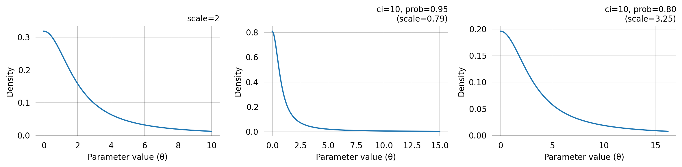
HalfCauchyPrior

A half-Cauchy prior with support on (0, \infty). Its heavy tails make it a popular weakly informative prior for scale and rate parameters — it concentrates mass near zero but allows for large values.

f(\theta) = \frac{2}{\pi \, \gamma \left(1 + (\theta/\gamma)^2\right)}, \quad \theta > 0

It can be specified via the scale parameter \gamma directly, or via a credible-interval upper bound.

fig, axes = plt.subplots(1, 3, figsize=(12, 3))

# 1. Scale parameter
h1 = HalfCauchyPrior(scale=2.0)
h1.plot(ax=axes[0], return_ax=True)
axes[0].set_title('scale=2')

# 2. 95% CI upper bound
h2 = HalfCauchyPrior(ci=10.0)
h2.plot(ax=axes[1], return_ax=True)
axes[1].set_title(f'ci=10, prob=0.95\n(scale={h2.scale:.2f})')

# 3. 80% CI upper bound
h3 = HalfCauchyPrior(ci=10.0, prob=0.80)
h3.plot(ax=axes[2], return_ax=True)
axes[2].set_title(f'ci=10, prob=0.80\n(scale={h3.scale:.2f})')

plt.tight_layout()

The CI specification says: “I believe there is a prob probability that the parameter is below ci.” A lower prob for the same ci implies a larger scale (heavier tail).

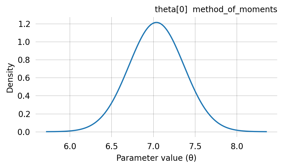
DataPrior

DataPrior constructs a data-informed prior automatically. Instead of specifying mean and spread by hand, it estimates them from the observed data using either method of moments (standard phase-type graphs) or probability matching (joint probability graphs). The graph type is detected automatically.

The result is a list of per-parameter GaussPrior objects (with None at fixed-parameter positions) that integrates directly with graph.svgd().

# Build a simple coalescent model
nr_samples = 4

@with_ipv([nr_samples]+[0]*(nr_samples-1))
def coalescent_1param(state):
    transitions = []
    for i in range(state.size):
        for j in range(i, state.size):            
            same = int(i == j)
            if same and state[i] < 2:
                continue
            if not same and (state[i] < 1 or state[j] < 1):
                continue 
            new = state.copy()
            new[i] -= 1
            new[j] -= 1
            new[i+j+1] += 1
            transitions.append([new, [state[i]*(state[j]-same)/(1+same)]])
    return transitions

graph = Graph(coalescent_1param)

true_theta = [7.0]
graph.update_weights(true_theta)
data = graph.sample(1000)

dp = DataPrior(graph, data, sd=2.0)
print(dp)
print(f"Method:    {dp.method}")
print(f"Theta:     {dp.theta}")
print(f"Std:       {dp.std}")
print(f"Converged: {dp.success}")

DataPrior(method=method_of_moments, converged, theta=[7.0386])
Method:    method_of_moments
Theta:     [7.03858073]
Std:       [0.16438664]
Converged: True

dp.plot()

DataPrior is iterable — you can inspect individual per-parameter priors and pass it directly to graph.svgd() as the prior argument:

# Inspect per-parameter priors
print(f"Number of parameters: {len(dp)}")
for i, p in enumerate(dp):
    if p is not None:
        print(f"  theta[{i}]: GaussPrior(mean={p.mu:.3f}, std={p.sigma:.3f})")
    else:
        print(f"  theta[{i}]: None (fixed)")

Number of parameters: 1
  theta[0]: GaussPrior(mean=7.039, std=0.329)

# Use directly with SVGD
svgd = graph.svgd(data, prior=dp, optimizer=Adam(0.25))
svgd.summary()

Parameter  Fixed      MAP        Mean       SD         HPD 95% lo   HPD 95% hi  
0          No         7.0287     6.9786     0.1275     6.6600       7.0866      

Particles: 24, Iterations: 100

DataPrior parameters:

Parameter	Type	Default	Description
graph	Graph	—	Parameterized graph
observed_data	array	—	Observed data
sd	float	2.0	Multiplier on the asymptotic standard error for the prior width
fixed	list	None	(index, value) tuples for fixed parameters
nr_moments	int	None	Number of moments (standard graphs only)
rewards	array	None	Reward vectors (standard graphs only)
theta_dim	int	None	Number of parameters (auto-detected)
theta_init	array	None	Initial guess for the free parameters
discrete	bool	None	Discrete or continuous model (auto-detected)
verbose	bool	False	Print progress

The sd parameter controls how wide the resulting Gaussian priors are relative to the estimation uncertainty. A larger value gives a more permissive prior:

• sd=1: Tight prior, trusts the MoM estimate closely
• sd=2 (default): Balanced
• sd=3–5: Wide prior, uses MoM only as a rough guide

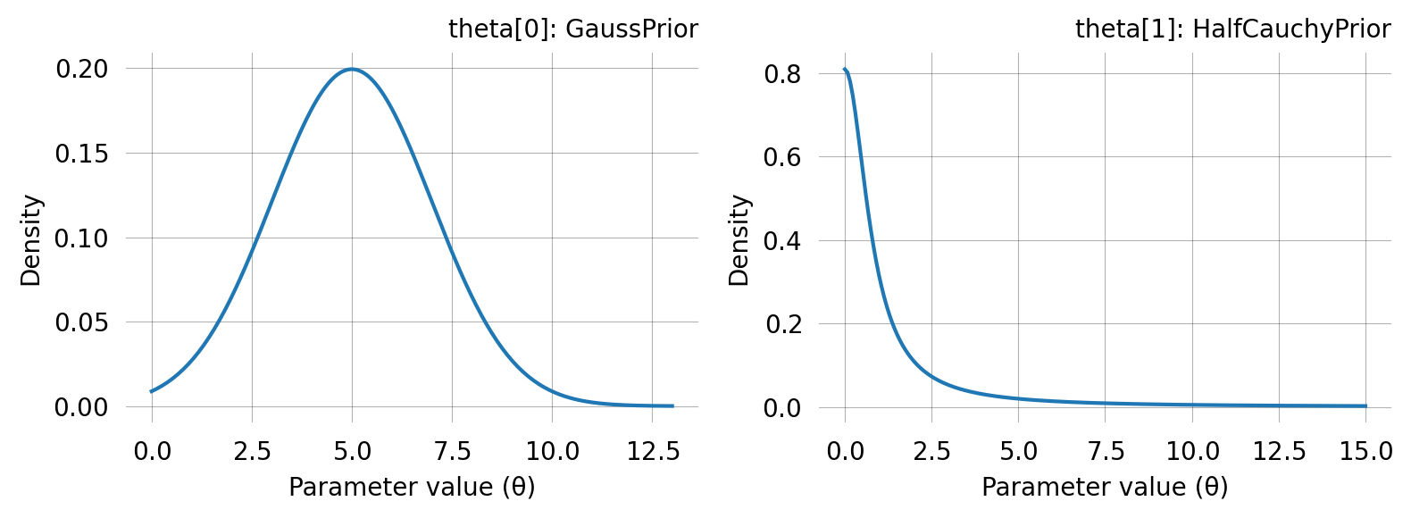
Per-parameter priors

When a model has multiple parameters, you can assign a different prior to each one by passing a list of prior objects to graph.svgd(). Use None at positions corresponding to fixed parameters:

per_param_priors = [
    GaussPrior(mean=5.0, std=2.0),   # theta[0]
    HalfCauchyPrior(ci=10.0),        # theta[1]
]

fig, axes = plt.subplots(1, 2, figsize=(8, 3))
per_param_priors[0].plot(ax=axes[0], return_ax=True)
axes[0].set_title('theta[0]: GaussPrior')
per_param_priors[1].plot(ax=axes[1], return_ax=True)
axes[1].set_title('theta[1]: HalfCauchyPrior')
plt.tight_layout()

Step size schedules

The step size (learning rate) controls how far particles move at each SVGD iteration. A step size that is too large causes oscillation; too small causes slow convergence. Schedules let you vary the step size over the course of optimisation.

Pass a schedule to graph.svgd() via the learning_rate parameter, or to an optimizer like Adam(learning_rate=schedule).

Class	Behaviour
ConstantStepSize	Fixed step size throughout
ExpStepSize	Exponential decay from a first to a last value
WarmupExpStepSize	Linear ramp-up then exponential decay
AdaptiveStepSize	Adjusts based on particle spread

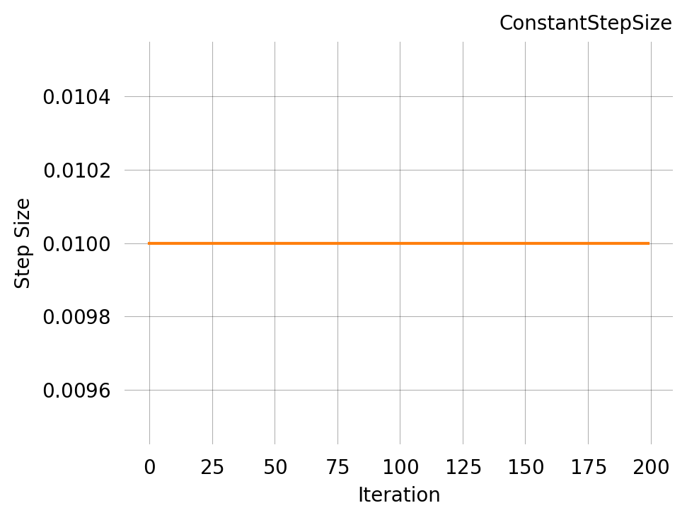
ConstantStepSize

The simplest schedule: the same step size at every iteration. This is also the implicit default when you pass a plain number as the learning_rate.

const = ConstantStepSize(0.01)
print(f"Step at iteration 0:   {const(0)}")
print(f"Step at iteration 500: {const(500)}")

const.plot(200)

Step at iteration 0:   0.01
Step at iteration 500: 0.01

Parameter	Type	Default	Description
step_size	float	0.01	Fixed step size

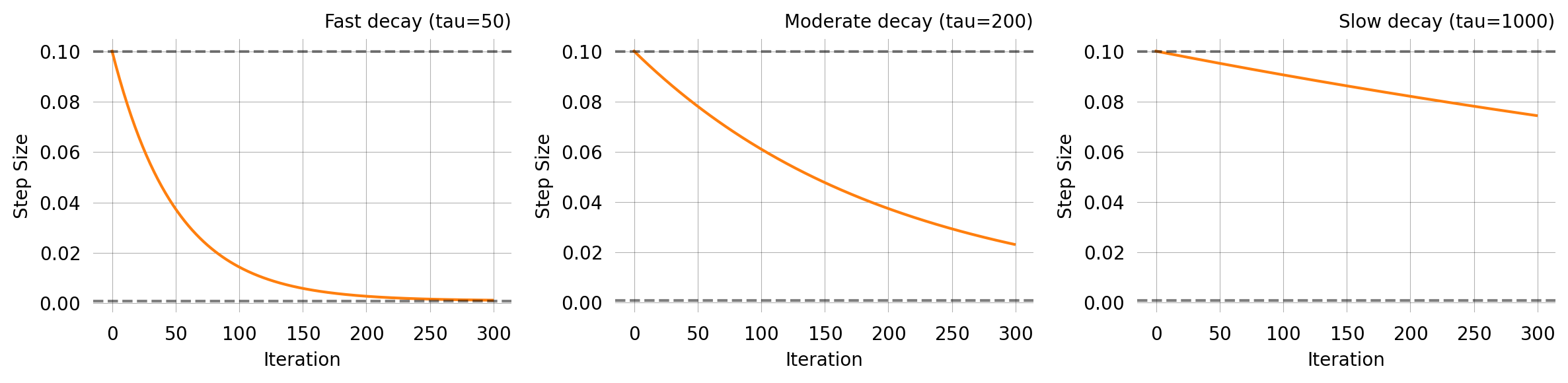
ExpStepSize

Exponential decay from first_step to last_step with time constant tau:

\eta(t) = \eta_0 \, e^{-t/\tau} + \eta_\infty \left(1 - e^{-t/\tau}\right)

At t = \tau, roughly 63% of the decay has occurred. This is the most commonly used schedule — start with a large step to explore, then settle down for fine-tuning.

fig, axes = plt.subplots(1, 3, figsize=(12, 3))

# Fast decay
s1 = ExpStepSize(first_step=0.1, last_step=0.001, tau=50.0)
s1.plot(300, ax=axes[0], return_ax=True)
axes[0].set_title('Fast decay (tau=50)')

# Moderate decay
s2 = ExpStepSize(first_step=0.1, last_step=0.001, tau=200.0)
s2.plot(300, ax=axes[1], return_ax=True)
axes[1].set_title('Moderate decay (tau=200)')

# Slow decay
s3 = ExpStepSize(first_step=0.1, last_step=0.001, tau=1000.0)
s3.plot(300, ax=axes[2], return_ax=True)
axes[2].set_title('Slow decay (tau=1000)')

plt.tight_layout()

Parameter	Type	Default	Description
first_step	float	0.01	Step size at iteration 0
last_step	float	1e-6	Asymptotic step size
tau	float	1000.0	Decay time constant (63% decay at t = \tau)

WarmupExpStepSize

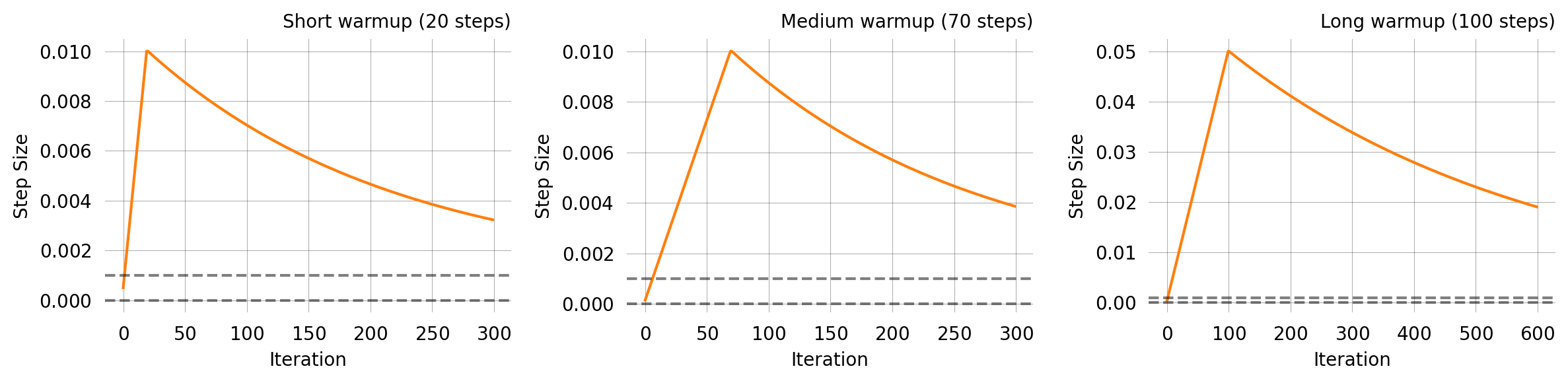
A linear ramp-up phase followed by exponential decay. This is useful with Adam and other adaptive optimizers where moment estimates are poorly calibrated in the first few iterations — a warmup prevents large early updates.

\eta(t) = \begin{cases} \eta_{\text{peak}} \cdot \frac{t+1}{T_{\text{warmup}}} & t < T_{\text{warmup}} \\ \eta_{\text{peak}} \, e^{-(t - T_{\text{warmup}})/\tau} + \eta_\infty \left(1 - e^{-(t - T_{\text{warmup}})/\tau}\right) & t \geq T_{\text{warmup}} \end{cases}

fig, axes = plt.subplots(1, 3, figsize=(12, 3))

# Short warmup
w1 = WarmupExpStepSize(peak_lr=0.01, warmup_steps=20, last_lr=0.001, tau=200.0)
w1.plot(300, ax=axes[0], return_ax=True)
axes[0].set_title('Short warmup (20 steps)')

# Medium warmup
w2 = WarmupExpStepSize(peak_lr=0.01, warmup_steps=70, last_lr=0.001, tau=200.0)
w2.plot(300, ax=axes[1], return_ax=True)
axes[1].set_title('Medium warmup (70 steps)')

# Long warmup, high peak
w3 = WarmupExpStepSize(peak_lr=0.05, warmup_steps=100, last_lr=0.001, tau=500.0)
w3.plot(600, ax=axes[2], return_ax=True)
axes[2].set_title('Long warmup (100 steps)')

plt.tight_layout()

Parameter	Type	Default	Description
peak_lr	float	0.001	Maximum learning rate at end of warmup
warmup_steps	int	100	Number of linear warmup iterations
last_lr	float	1e-6	Asymptotic learning rate
tau	float	1000.0	Decay time constant after warmup

AdaptiveStepSize

Adjusts the step size dynamically based on particle spread. When particles are too concentrated the step size increases; when too dispersed it decreases. This is a simple heuristic that does not require tuning a decay schedule, but its behaviour depends on the optimisation trajectory.

adaptive = AdaptiveStepSize(base_step=0.01, kl_target=0.1, adjust_rate=0.1)
print(f"Base step: {adaptive.base_step}")
print(f"Without particles: {adaptive(0):.4f}")

# Simulate concentrated particles
concentrated = jnp.array([[1.0], [1.01], [0.99]])
print(f"Concentrated particles: {adaptive(1, concentrated):.4f} (increases)")

# Simulate spread particles
spread = jnp.array([[1.0], [10.0], [100.0]])
print(f"Spread particles: {adaptive(2, spread):.4f} (decreases)")

Base step: 0.01
Without particles: 0.0100
Concentrated particles: 0.0110 (increases)
Spread particles: 0.0099 (decreases)

Parameter	Type	Default	Description
base_step	float	0.01	Initial step size
kl_target	float	0.1	Target log-spread of particles
adjust_rate	float	0.1	Rate of multiplicative adjustment per step

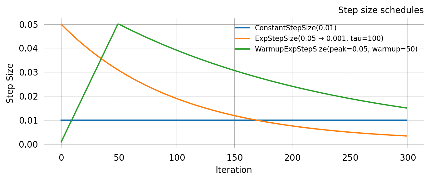
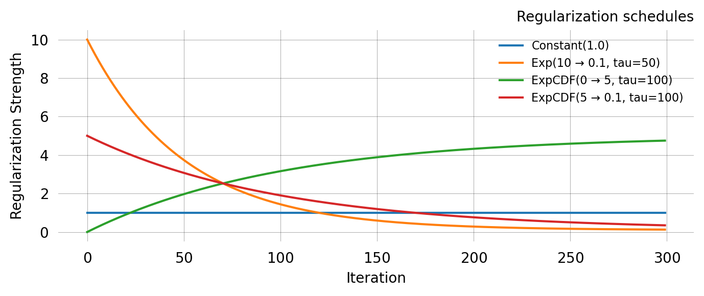
Comparison

All four schedules on the same axes for a 300-iteration run:

nr_iter = 300
iters = np.arange(nr_iter)

schedules = {
    'ConstantStepSize(0.01)': ConstantStepSize(0.01),
    'ExpStepSize(0.05 → 0.001, tau=100)': ExpStepSize(0.05, 0.001, 100.0),
    'WarmupExpStepSize(peak=0.05, warmup=50)': WarmupExpStepSize(0.05, 50, 0.001, 200.0),
}

fig, ax = plt.subplots(figsize=(7, 3))
for label, sched in schedules.items():
    vals = [float(sched(i)) for i in iters]
    ax.plot(iters, vals, label=label)

ax.set_xlabel('Iteration')
ax.set_ylabel('Step Size')
ax.set_title('Step size schedules')
ax.legend(fontsize=8)
plt.tight_layout()

Regularization schedules

Moment regularization adds a penalty term to the SVGD objective that encourages the model moments at the current parameter values to match the empirical moments. This is controlled by the regularization parameter in graph.svgd() and requires specifying nr_moments.

Strong regularization early in optimisation helps guide particles into a reasonable region; reducing it later lets the likelihood dominate for fine-tuning.

Class	Behaviour
ConstantRegularization	Fixed regularization strength
ExpRegularization	Exponential decay from first to last value
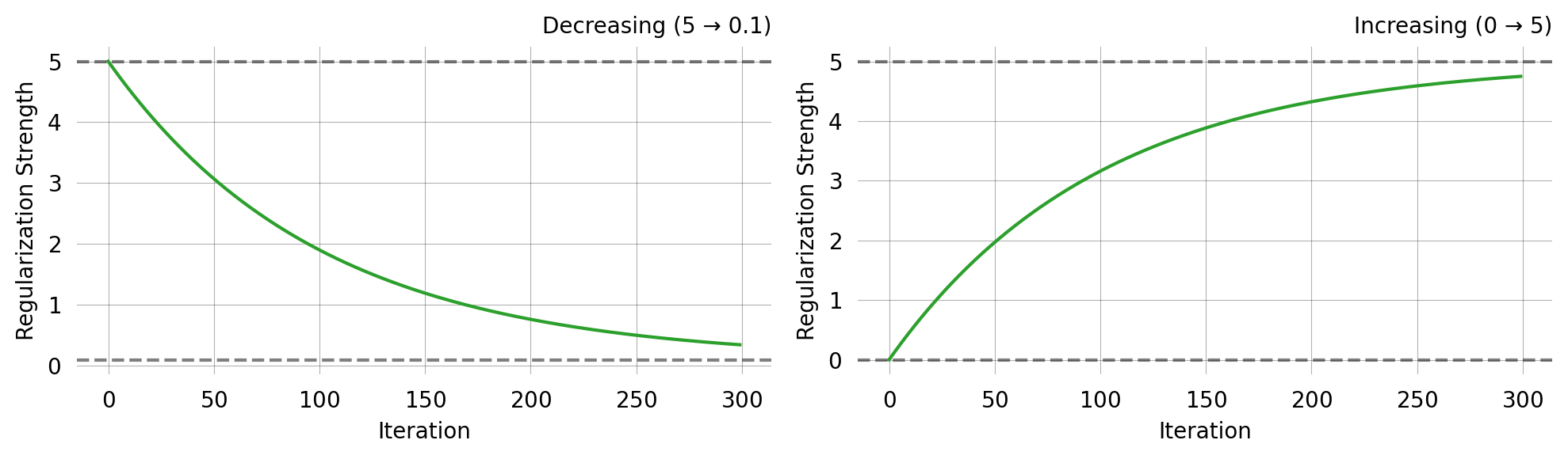
ExponentialCDFRegularization	Smooth CDF-based transition (works for both increasing and decreasing)

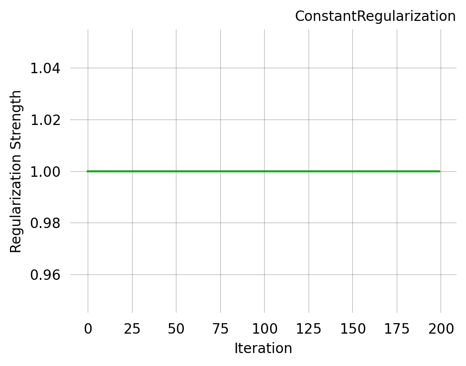
ConstantRegularization

A fixed regularization strength throughout optimisation.

const_reg = ConstantRegularization(1.0)
print(f"Strength at iteration 0:   {const_reg(0)}")
print(f"Strength at iteration 500: {const_reg(500)}")

const_reg.plot(200)

Strength at iteration 0:   1.0
Strength at iteration 500: 1.0

Parameter	Type	Default	Description
regularization	float	0.0	Fixed regularization strength

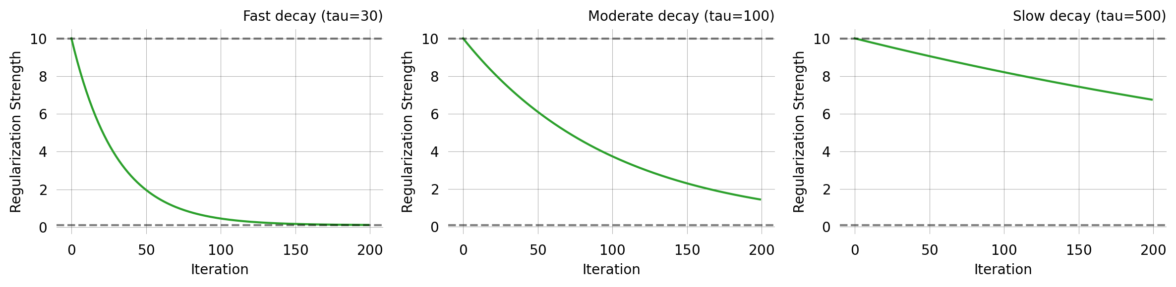
ExpRegularization

Exponential decay, identical in form to ExpStepSize:

\lambda(t) = \lambda_0 \, e^{-t/\tau} + \lambda_\infty \left(1 - e^{-t/\tau}\right)

Start with strong regularization to guide particles, then reduce to let the likelihood dominate.

fig, axes = plt.subplots(1, 3, figsize=(12, 3))

r1 = ExpRegularization(first_reg=10.0, last_reg=0.1, tau=30.0)
r1.plot(200, ax=axes[0], return_ax=True)
axes[0].set_title('Fast decay (tau=30)')

r2 = ExpRegularization(first_reg=10.0, last_reg=0.1, tau=100.0)
r2.plot(200, ax=axes[1], return_ax=True)
axes[1].set_title('Moderate decay (tau=100)')

r3 = ExpRegularization(first_reg=10.0, last_reg=0.1, tau=500.0)
r3.plot(200, ax=axes[2], return_ax=True)
axes[2].set_title('Slow decay (tau=500)')

plt.tight_layout()

Parameter	Type	Default	Description
first_reg	float	1.0	Regularization strength at iteration 0
last_reg	float	0.0	Asymptotic regularization strength
tau	float	1000.0	Decay time constant

ExponentialCDFRegularization

Uses the exponential CDF for a smooth S-curve transition:

\lambda(t) = \lambda_0 + (\lambda_\infty - \lambda_0) \left(1 - e^{-t/\tau}\right)

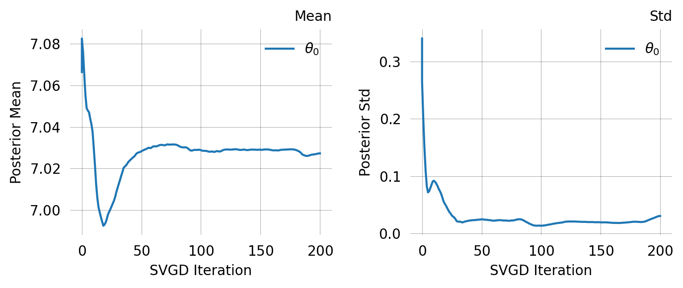
This is mathematically equivalent to ExpRegularization for decreasing schedules, but the parameterisation makes it equally natural for increasing schedules — useful for progressive regularization where you start with pure likelihood and gradually add moment matching.

fig, axes = plt.subplots(1, 2, figsize=(10, 3))

# Decreasing (same as ExpRegularization)
c1 = ExponentialCDFRegularization(first_reg=5.0, last_reg=0.1, tau=100.0)
c1.plot(300, ax=axes[0], return_ax=True)
axes[0].set_title('Decreasing (5 → 0.1)')

# Increasing — start with likelihood only, add regularization later
c2 = ExponentialCDFRegularization(first_reg=0.0, last_reg=5.0, tau=100.0)
c2.plot(300, ax=axes[1], return_ax=True)
axes[1].set_title('Increasing (0 → 5)')

plt.tight_layout()

Parameter	Type	Default	Description
first_reg	float	0.0	Regularization strength at iteration 0
last_reg	float	1.0	Asymptotic regularization strength
tau	float	1000.0	Transition time constant (63% of transition at t = \tau)

Comparison

nr_iter = 300
iters = np.arange(nr_iter)

reg_schedules = {
    'Constant(1.0)': ConstantRegularization(1.0),
    'Exp(10 → 0.1, tau=50)': ExpRegularization(10.0, 0.1, 50.0),
    'ExpCDF(0 → 5, tau=100)': ExponentialCDFRegularization(0.0, 5.0, 100.0),
    'ExpCDF(5 → 0.1, tau=100)': ExponentialCDFRegularization(5.0, 0.1, 100.0),
}

fig, ax = plt.subplots(figsize=(7, 3))
for label, sched in reg_schedules.items():
    vals = [float(sched(i)) for i in iters]
    ax.plot(iters, vals, label=label)

ax.set_xlabel('Iteration')
ax.set_ylabel('Regularization Strength')
ax.set_title('Regularization schedules')
ax.legend(fontsize=8)
plt.tight_layout()

Putting it together

A typical SVGD call combining priors and schedules:

svgd = graph.svgd(
    data,
    prior=DataPrior(graph, data, sd=2.0),
    optimizer=Adam(
        learning_rate=ExpStepSize(first_step=0.1, last_step=0.01, tau=30.0),
    ),
    # regularization=ExpRegularization(first_reg=5.0, last_reg=0.1, tau=20.0),
    # nr_moments=2,
    n_iterations=200,
)
svgd.summary()
svgd.plot_convergence() ;

Parameter  Fixed      MAP        Mean       SD         HPD 95% lo   HPD 95% hi  
0          No         7.0294     7.0273     0.0306     6.9664       7.1014      

Particles: 24, Iterations: 200

TipGeneral guidance

• Prior: Start with DataPrior for an automatic data-informed prior. Fall back to GaussPrior(ci=...) if you have domain knowledge, or HalfCauchyPrior for weakly informative priors on scale parameters.
• Step size: Adam(0.25) with the default constant step size works well for many problems. If convergence is unsteady, try ExpStepSize or WarmupExpStepSize.
• Regularization: Often not needed if the prior is informative. Use ExpRegularization to stabilise early iterations in difficult models.