from phasic import Graph, with_ipv, StateIndexer, Property, set_log_level # ALWAYS import phasic first to set jax backend correctly
import sys
import numpy as np
import matplotlib.pyplot as plt
import seaborn as sns
%config InlineBackend.figure_format = 'svg'
from vscodenb import set_vscode_theme

np.random.seed(42)
set_vscode_theme()
sns.set_palette('tab10')Parameterized models
We can parameterize the edges to easily update the weights of the edge. We do this by assigning a coefficient vector to the edge instead of a rate.
Once we have built the graph, we set the can set the model parameters using a vector of scalars with the same length as those assigned to the graph edges. This changes the weight of each edge to the inner sum of the edge vector and the parameter vector. E.g. if the state is x1, x2 and the parameters are p1, p2, then the weight of the edge become x1*p1+x2*p2.
Continuous phase-type distributions
To parameterize the ARG model above, we remove the keyword arguments N and R, assume their values are 1 so that the the coalescent rate is no longer a fixed rate
state[i]*(state[j]-same)/(1+same) / N
but the a coefficient vector:
[[state[i]*(state[j]-same)/(1+same), 0]
Similarly the recombination rate is no longer R but [0, 1].
A parameter vector of [1/N, R] will then produce the appropriate edge weights.
nr_samples = 4
indexer = StateIndexer(descendants=[
    Property('loc1', max_value=nr_samples),
    Property('loc2', max_value=nr_samples)
])

initial = [0] * indexer.state_length
initial[indexer.props_to_index(loc1=1, loc2=1)] = nr_samples

@with_ipv(initial)
def two_locus_arg_2param(state, indexer=None): # <- changed

    transitions = []
    if state.sum() <= 1: return transitions

    for i in range(indexer.state_length):
        if state[i] == 0: continue
        pi = indexer.index_to_props(i)

        for j in range(i, indexer.state_length):
            if state[j] == 0: continue
            pj = indexer.index_to_props(j)

            same = int(i == j)
            if same and state[i] < 2:
                continue
            if not same and (state[i] < 1 or state[j] < 1):
                continue
            child = state.copy()
            child[i] -= 1
            child[j] -= 1
            loc1 = pi.descendants.loc1 + pj.descendants.loc1
            loc2 = pi.descendants.loc2 + pj.descendants.loc2
            if loc1 <= nr_samples and loc2 <= nr_samples:
                child[indexer.props_to_index(loc1=loc1, loc2=loc2)] += 1
                transitions.append([child, [state[i]*(state[j]-same)/(1+same), 0]]) # <- changed

        if state[i] > 0 and pi.descendants.loc1 > 0 and pi.descendants.loc2 > 0:
            child = state.copy()
            child[i] -= 1
            child[indexer.props_to_index(loc1=pi.descendants.loc1, loc2=0)] += 1
            child[indexer.props_to_index(loc1=0, loc2=pi.descendants.loc2)] += 1
            transitions.append([child, [0, 1]])                                 # <- changed

    return transitions


graph = Graph(two_locus_arg_2param, indexer=indexer)
If you forget, you can get the number of parameters by calling:
# graph.param_length()Having defined the graph with edge coefficients rather than fixed weights, we can now update the weights with specific parameter values and compute expectations. Here, we set the coalescence rate to (1/N) and the recombination rate to (R) and compute the expectation:
graph.update_weights([1/3, 5])
graph.expectation()8.737804379412143The new weights are computed as the the dot product of the edge coefficients and the vector of parameters passed to update_weights (parameters*coefficients). This covers most use cases, but for full flexibility you can pass a callback function callback(parameters, coefficients) -> weight. The example below is the same as the default behaviour:
graph.update_weights([1/3, 5], callback = lambda param, coef: np.sum(param * coef))
graph.expectation()8.737804379412143Now we can compute moments and distributions for different values of N and R without reconstructing the graph:
R_values = [1, 2, 1, 2, 1, 2]
N_values = [1, 1, 1.5, 1.5, 2, 2]

for N, R in zip(N_values, R_values):
    graph.update_weights([1/N, R])
    print(f'N:{N:<5} R:{R:<4} Mean: {graph.expectation():.4f}   Var:{graph.variance():.4f}')
N:1 R:1 Mean: 2.0091 Var:2.0644
N:1 R:2 Mean: 2.2949 Var:2.3298
N:1.5 R:1 Mean: 3.2565 Var:5.0348
N:1.5 R:2 Mean: 3.7032 Var:5.4037
N:2 R:1 Mean: 4.5897 Var:9.3191
N:2 R:2 Mean: 5.1655 Var:9.6596x = np.arange(0, 10, 0.1)
for N, R in zip(N_values, R_values):
graph.update_weights([1/N, R])
plt.plot(x, graph.pdf(x), label=f'N: {N} R: {R}')
plt.xlabel('Reward (TMRCA)')
plt.legend()
plt.show()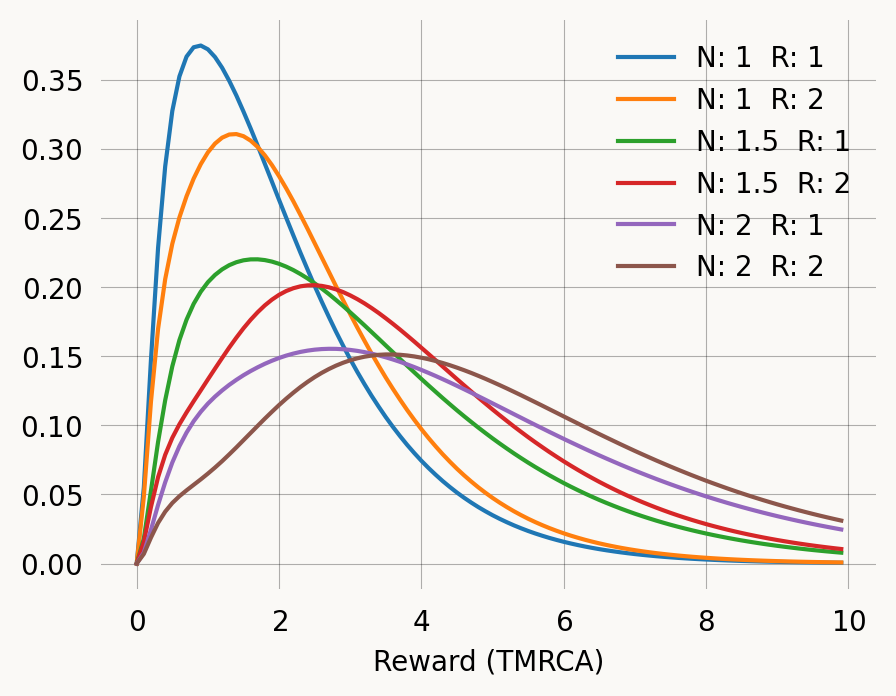
When using the callback argument, the parameter vector can be shorter than the coefficient vectors. Just pass the param_length keyword argument to the Graph constructor. Allowing for more coefficients s handy if you need to pass more information to the callback function in order to update edge weights.
Discrete phase-type distributions
Let us go back to the simpler coalescent model as an example of a discrete parameterized model.
@with_ipv([nr_samples]+[0]*(nr_samples-1))
def coalescent_2param(state):
    transitions = []
    for i in range(state.size):
        for j in range(i, state.size):
            same = int(i == j)
            if same and state[i] < 2:
                continue
            if not same and (state[i] < 1 or state[j] < 1):
                continue
            new = state.copy()
            new[i] -= 1
            new[j] -= 1
            new[i+j+1] += 1
            transitions.append((new, [state[i]*(state[j]-same)/(1+same), 0]))
    return transitions

mutation_graph = Graph(coalescent_2param)

def mutation_rate(state):
    nr_lineages = sum(state)
    return [0, nr_lineages]

rewards = mutation_graph.discretize(mutation_rate)

print("Discrete rewards (indices of AUX vertices):", rewards)
mutation_graph.plot()
Discrete rewards (indices of AUX vertices): [0 0 0 0 0 0 1 1 1 1]
mutation_graph.update_weights([3, 2])
rt_graph = mutation_graph.reward_transform(rewards)
rt_graph.plot()
mutation_graph.update_weights([3, 2])
rt_graph = mutation_graph.reward_transform(rewards)
rt_graph.pdf(2)0.14830307025146516mutation_graph.plot()
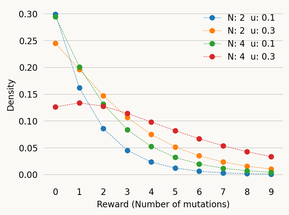
rt_graph.expectation(), mutation_graph.expectation(rewards)(2.444444444444444, 2.444444444444444)rt_graph.variance(), mutation_graph.variance(rewards)(7.30864197530864, 4.864197530864198)N_values = [2, 2, 4, 4, ]
u_values = [0.1, 0.3, 0.1, 0.3]
x = np.arange(0, 10, 1)
for N, u in zip(N_values, u_values):
mutation_graph.update_weights([1/N, u])
rt_graph = mutation_graph.reward_transform(rewards)
sns.pointplot(x=x, y=rt_graph.pdf(x), label=f'N: {N} u: {u}',
linestyle='dashed', markers='o',
markersize=6, linewidth=0.5)
plt.xlabel('Reward (Number of mutations)')
plt.ylabel('Density')
plt.legend()
plt.show()