Priors and schedules

This page covers the prior distributions, step size schedules, and regularization schedules available for use with SVGD inference.

from phasic import (
    Graph, with_ipv,
    # Priors
    GaussPrior, HalfCauchyPrior, DataPrior,
    # Step size schedules
    ConstantStepSize, ExpStepSize, AdaptiveStepSize, WarmupExpStepSize,
    # Regularization schedules
    ConstantRegularization, ExpRegularization, ExponentialCDFRegularization,
    # Optimizers (for examples)
    Adam,
) # ALWAYS import phasic first to set jax backend correctly
import numpy as np
import jax.numpy as jnp
import matplotlib.pyplot as plt
import seaborn as sns

np.random.seed(42)
try:
    from vscodenb import set_vscode_theme
    set_vscode_theme()
except ImportError:
    pass
sns.set_palette('tab10')

Priors

GaussPrior

A Gaussian (normal) prior centred on a point estimate with a given spread. It can be specified either by the mean and standard deviation or by a credible interval. E.g., “I believe the parameter is between 2 and 8 with 95% probability” translates directly to GaussPrior(ci=(2, 8)). The two specifications are equivalent: a 95% credible interval [low, high] maps to mean = (low + high) / 2 and std = (high - low) / (2 * z_0.975).

fig, axes = plt.subplots(1, 3, figsize=(12, 3))

# 1. Mean + std
p1 = GaussPrior(mean=5.0, std=1.5)
p1.plot(ax=axes[0], return_ax=True)
axes[0].set_title(f'mean=5, std=1.5')

# 2. 95% credible interval
p2 = GaussPrior(ci=(2.0, 8.0))
p2.plot(ax=axes[1], return_ax=True)
axes[1].set_title(f'ci=[2, 8], prob=0.95')

# 3. 80% credible interval (tighter)
p3 = GaussPrior(ci=(3.0, 7.0), prob=0.80)
p3.plot(ax=axes[2], return_ax=True)
axes[2].set_title(f'ci=[3, 7], prob=0.80')

plt.tight_layout()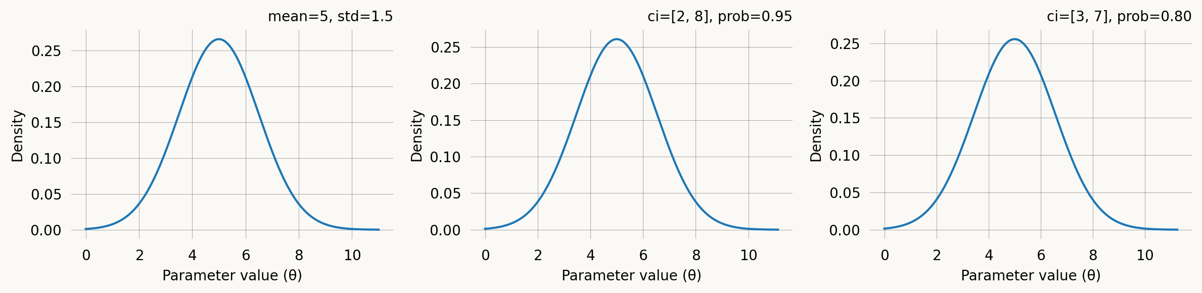

HalfCauchyPrior

A half-Cauchy prior with support on (0, \infty). Its heavy tails make it a popular weakly informative prior for scale and rate parameters. Concentrates mass near zero but allows for large values.

f(\theta) = \frac{2}{\pi \, \gamma \left(1 + (\theta/\gamma)^2\right)}, \quad \theta > 0

It can be specified via the scale parameter \gamma directly, or via a credible-interval upper bound. The CI specification says: “I believe there is a prob probability that the parameter is below ci.” A lower prob for the same ci implies a larger scale (heavier tail).

fig, axes = plt.subplots(1, 3, figsize=(12, 3))

# 1. Scale parameter
h1 = HalfCauchyPrior(scale=2.0)
h1.plot(ax=axes[0], return_ax=True)
axes[0].set_title('scale=2')

# 2. 95% CI upper bound
h2 = HalfCauchyPrior(ci=10.0)
h2.plot(ax=axes[1], return_ax=True)
axes[1].set_title(f'ci=10, prob=0.95\n(scale={h2.scale:.2f})')

# 3. 80% CI upper bound
h3 = HalfCauchyPrior(ci=10.0, prob=0.80)
h3.plot(ax=axes[2], return_ax=True)
axes[2].set_title(f'ci=10, prob=0.80\n(scale={h3.scale:.2f})')

plt.tight_layout()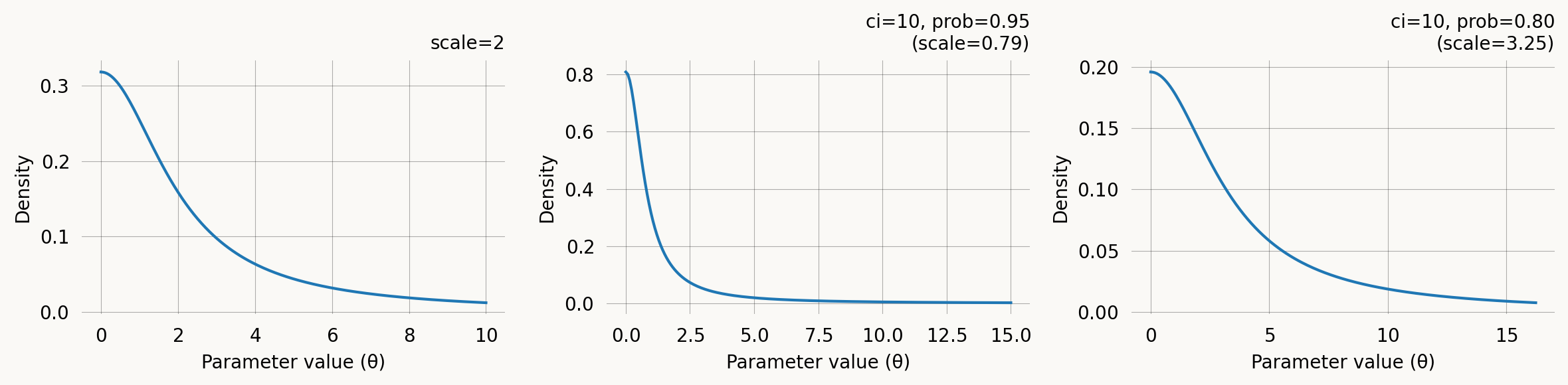

DataPrior

DataPrior constructs a data-informed prior automatically. Instead of specifying mean and spread by hand, it estimates them from the observed data using either method of moments (standard phase-type graphs) or probability matching (joint probability graphs). The graph type is detected automatically. The result is a list of per-parameter GaussPrior objects (with None at fixed-parameter positions) that integrates directly with graph.svgd().

# Build a simple coalescent model
nr_samples = 4

@with_ipv([nr_samples]+[0]*(nr_samples-1))
def coalescent_1param(state):
    transitions = []
    for i in range(state.size):
        for j in range(i, state.size):            
            same = int(i == j)
            if same and state[i] < 2:
                continue
            if not same and (state[i] < 1 or state[j] < 1):
                continue 
            new = state.copy()
            new[i] -= 1
            new[j] -= 1
            new[i+j+1] += 1
            transitions.append([new, [state[i]*(state[j]-same)/(1+same)]])
    return transitions

graph = Graph(coalescent_1param)

true_theta = [7.0]
graph.update_weights(true_theta)
data = graph.sample(1000)

dp = DataPrior(graph, data, sd=2.0)
print(dp)
print(f"Method:    {dp.method}")
print(f"Theta:     {dp.theta}")
print(f"Std:       {dp.std}")
print(f"Converged: {dp.success}")

DataPrior(method=method_of_moments, converged, theta=[6.8063])
Method:    method_of_moments
Theta:     [6.80628673]
Std:       [0.14097399]
Converged: True

dp.plot()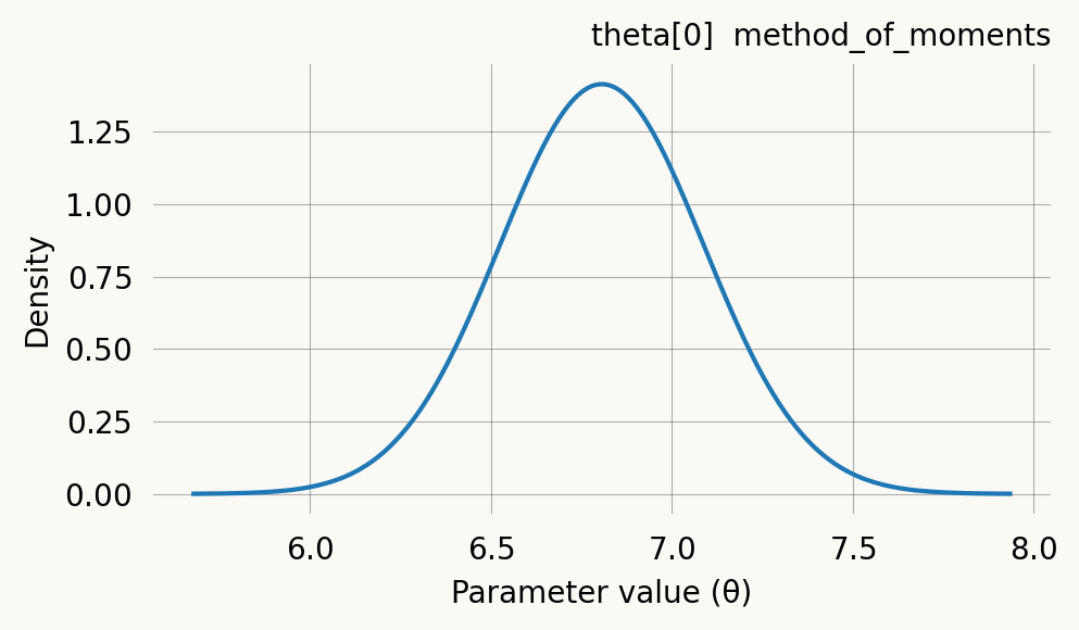

DataPrior is iterable — you can inspect individual per-parameter priors and pass it directly to graph.svgd() as the prior argument:

# Inspect per-parameter priors
print(f"Number of parameters: {len(dp)}")
for i, p in enumerate(dp):
    if p is not None:
        print(f"  theta[{i}]: GaussPrior(mean={p.mu:.3f}, std={p.sigma:.3f})")
    else:
        print(f"  theta[{i}]: None (fixed)")

Number of parameters: 1
  theta[0]: GaussPrior(mean=6.806, std=0.282)

# Use directly with SVGD
svgd = graph.svgd(data, prior=dp, optimizer=Adam(0.25))
svgd.summary()

Parameter  Fixed      MAP        Mean       SD         HPD 95% lo   HPD 95% hi  
0          No         6.7121     6.7367     0.1025     6.5919       6.9032      

Particles: 24, Iterations: 100

See the API documentation on DataPrior for all parameters.

Per-parameter priors

When a model has multiple parameters, you can assign a different prior to each one by passing a list of prior objects to graph.svgd(). Use None at positions corresponding to fixed parameters:

per_param_priors = [
    GaussPrior(mean=5.0, std=2.0),   # theta[0]
    HalfCauchyPrior(ci=10.0),        # theta[1]
]

fig, axes = plt.subplots(1, 2, figsize=(8, 3))
per_param_priors[0].plot(ax=axes[0], return_ax=True)
axes[0].set_title('theta[0]: GaussPrior')
per_param_priors[1].plot(ax=axes[1], return_ax=True)
axes[1].set_title('theta[1]: HalfCauchyPrior')
plt.tight_layout()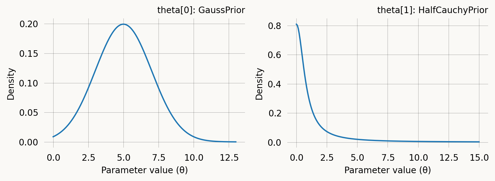

Step size schedules

The step size (learning rate) controls how far particles move at each SVGD iteration. A step size that is too large causes oscillation; too small causes slow convergence. Schedules let you vary the step size over the course of optimization. Pass a schedule to graph.svgd() via the learning_rate parameter, or to an optimizer like Adam(learning_rate=schedule).

ConstantStepSize

The simplest schedule: the same step size at every iteration. This is also the implicit default when you pass a plain number as the learning_rate.

const = ConstantStepSize(0.01)
print(f"Step at iteration 0:   {const(0)}")
print(f"Step at iteration 500: {const(500)}")

const.plot(200)

Step at iteration 0:   0.01
Step at iteration 500: 0.01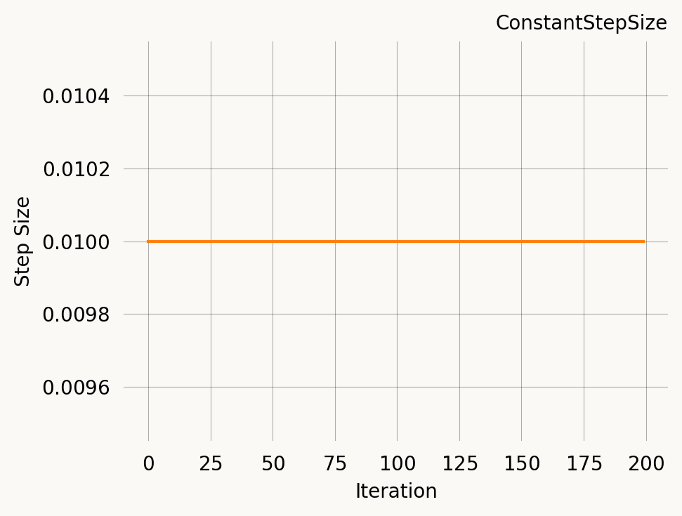

Se the API documentation for ConstantStepSize for all parameters.

ExpStepSize

Exponential decay from first_step to last_step with time constant tau:

\eta(t) = \eta_0 \, e^{-t/\tau} + \eta_\infty \left(1 - e^{-t/\tau}\right)

At t = \tau, roughly 63% of the decay has occurred. This is the most commonly used schedule — start with a large step to explore, then settle down for fine-tuning.

fig, axes = plt.subplots(1, 3, figsize=(12, 3))

# Fast decay
s1 = ExpStepSize(first_step=0.1, last_step=0.001, tau=50.0)
s1.plot(300, ax=axes[0], return_ax=True)
axes[0].set_title('Fast decay (tau=50)')

# Moderate decay
s2 = ExpStepSize(first_step=0.1, last_step=0.001, tau=200.0)
s2.plot(300, ax=axes[1], return_ax=True)
axes[1].set_title('Moderate decay (tau=200)')

# Slow decay
s3 = ExpStepSize(first_step=0.1, last_step=0.001, tau=1000.0)
s3.plot(300, ax=axes[2], return_ax=True)
axes[2].set_title('Slow decay (tau=1000)')

plt.tight_layout()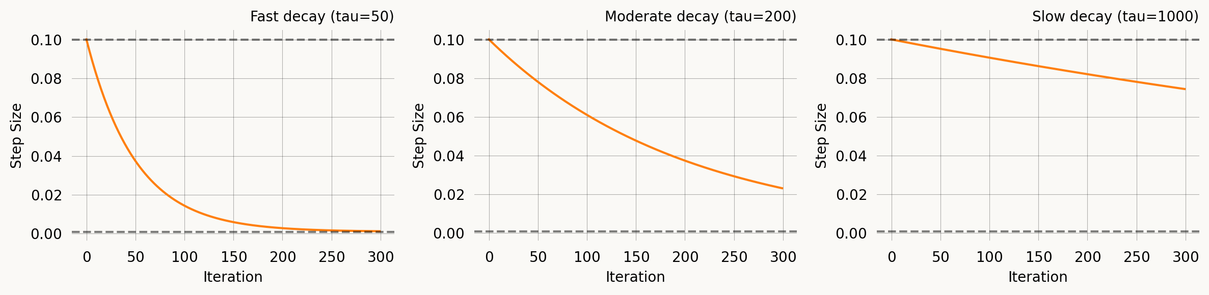

Se the API documentation for ExpStepSize for all parameters.

WarmupExpStepSize

A linear ramp-up phase followed by exponential decay. This is useful with Adam and other adaptive optimizers where moment estimates are poorly calibrated in the first few iterations — a warmup prevents large early updates.

\eta(t) = \begin{cases} \eta_{\text{peak}} \cdot \frac{t+1}{T_{\text{warmup}}} & t < T_{\text{warmup}} \\ \eta_{\text{peak}} \, e^{-(t - T_{\text{warmup}})/\tau} + \eta_\infty \left(1 - e^{-(t - T_{\text{warmup}})/\tau}\right) & t \geq T_{\text{warmup}} \end{cases}

fig, axes = plt.subplots(1, 3, figsize=(12, 3))

# Short warmup
w1 = WarmupExpStepSize(peak_lr=0.01, warmup_steps=20, last_lr=0.001, tau=200.0)
w1.plot(300, ax=axes[0], return_ax=True)
axes[0].set_title('Short warmup (20 steps)')

# Medium warmup
w2 = WarmupExpStepSize(peak_lr=0.01, warmup_steps=70, last_lr=0.001, tau=200.0)
w2.plot(300, ax=axes[1], return_ax=True)
axes[1].set_title('Medium warmup (70 steps)')

# Long warmup, high peak
w3 = WarmupExpStepSize(peak_lr=0.05, warmup_steps=100, last_lr=0.001, tau=500.0)
w3.plot(600, ax=axes[2], return_ax=True)
axes[2].set_title('Long warmup (100 steps)')

plt.tight_layout()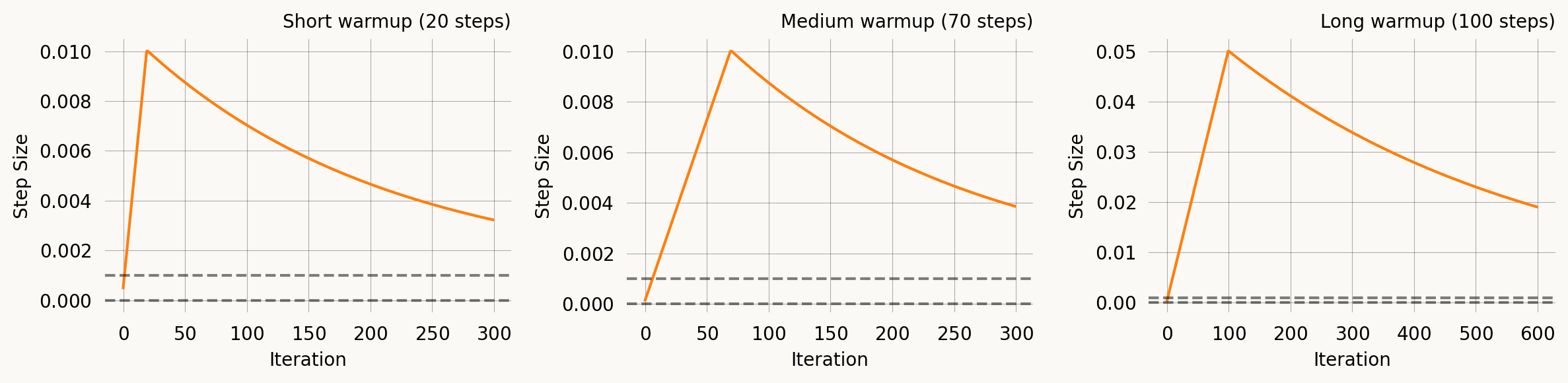

Se the API documentation for WarmupExpStepSize for all parameters.

AdaptiveStepSize

Adjusts the step size dynamically based on particle spread. When particles are too concentrated the step size increases; when too dispersed it decreases. This is a simple heuristic that does not require tuning a decay schedule, but its behaviour depends on the optimisation trajectory.

adaptive = AdaptiveStepSize(base_step=0.01, kl_target=0.1, adjust_rate=0.1)
print(f"Base step: {adaptive.base_step}")
print(f"Without particles: {adaptive(0):.4f}")

# Simulate concentrated particles
concentrated = jnp.array([[1.0], [1.01], [0.99]])
print(f"Concentrated particles: {adaptive(1, concentrated):.4f} (increases)")

# Simulate spread particles
spread = jnp.array([[1.0], [10.0], [100.0]])
print(f"Spread particles: {adaptive(2, spread):.4f} (decreases)")

Base step: 0.01
Without particles: 0.0100
Concentrated particles: 0.0110 (increases)
Spread particles: 0.0099 (decreases)

Se the API documentation for AdaptiveStepSize for all parameters.

Comparison

All four schedules on the same axes for a 300-iteration run:

nr_iter = 300
iters = np.arange(nr_iter)

schedules = {
    'ConstantStepSize(0.01)': ConstantStepSize(0.01),
    'ExpStepSize(0.05 → 0.001, tau=100)': ExpStepSize(0.05, 0.001, 100.0),
    'WarmupExpStepSize(peak=0.05, warmup=50)': WarmupExpStepSize(0.05, 50, 0.001, 200.0),
}

fig, ax = plt.subplots(figsize=(7, 3))
for label, sched in schedules.items():
    vals = [float(sched(i)) for i in iters]
    ax.plot(iters, vals, label=label)

ax.set_xlabel('Iteration')
ax.set_ylabel('Step Size')
ax.set_title('Step size schedules')
ax.legend(fontsize=8)
plt.tight_layout()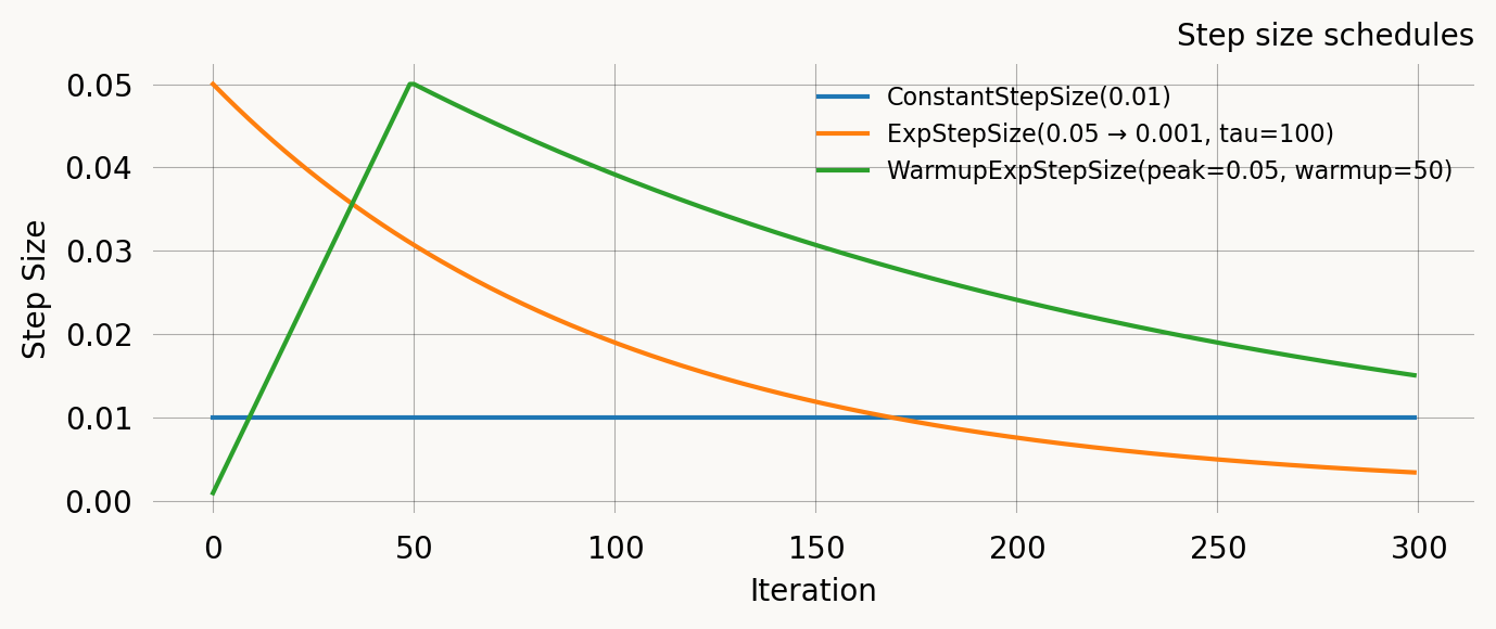

Regularization schedules

Moment regularization adds a penalty term to the SVGD objective that encourages the model moments at the current parameter values to match the empirical moments. This is controlled by the regularization parameter in graph.svgd() and requires specifying nr_moments. Strong regularization early in optimization helps guide particles into a reasonable region; reducing it later lets the likelihood dominate for fine-tuning.

ConstantRegularization

A fixed regularization strength throughout optimisation.

const_reg = ConstantRegularization(1.0)
print(f"Strength at iteration 0:   {const_reg(0)}")
print(f"Strength at iteration 500: {const_reg(500)}")

const_reg.plot(200)

Strength at iteration 0:   1.0
Strength at iteration 500: 1.0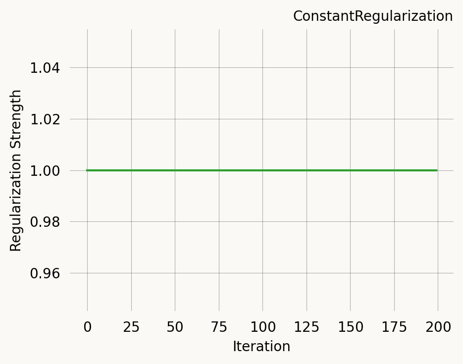

Se the API documentation for ConstantRegularization for all parameters.

ExpRegularization

Exponential decay, identical in form to ExpStepSize:

\lambda(t) = \lambda_0 \, e^{-t/\tau} + \lambda_\infty \left(1 - e^{-t/\tau}\right)

Start with strong regularization to guide particles, then reduce to let the likelihood dominate.

fig, axes = plt.subplots(1, 3, figsize=(12, 3))

r1 = ExpRegularization(first_reg=10.0, last_reg=0.1, tau=30.0)
r1.plot(200, ax=axes[0], return_ax=True)
axes[0].set_title('Fast decay (tau=30)')

r2 = ExpRegularization(first_reg=10.0, last_reg=0.1, tau=100.0)
r2.plot(200, ax=axes[1], return_ax=True)
axes[1].set_title('Moderate decay (tau=100)')

r3 = ExpRegularization(first_reg=10.0, last_reg=0.1, tau=500.0)
r3.plot(200, ax=axes[2], return_ax=True)
axes[2].set_title('Slow decay (tau=500)')

plt.tight_layout()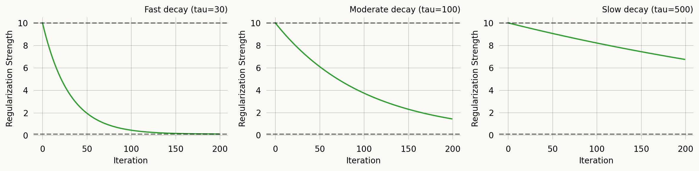

Se the API documentation for ExpRegularization for all parameters.

ExponentialCDFRegularization

Uses the exponential CDF for a smooth S-curve transition:

\lambda(t) = \lambda_0 + (\lambda_\infty - \lambda_0) \left(1 - e^{-t/\tau}\right)

This is mathematically equivalent to ExpRegularization for decreasing schedules, but the parameterisation makes it equally natural for increasing schedules — useful for progressive regularization where you start with pure likelihood and gradually add moment matching.

fig, axes = plt.subplots(1, 2, figsize=(10, 3))

# Decreasing (same as ExpRegularization)
c1 = ExponentialCDFRegularization(first_reg=5.0, last_reg=0.1, tau=100.0)
c1.plot(300, ax=axes[0], return_ax=True)
axes[0].set_title('Decreasing (5 → 0.1)')

# Increasing — start with likelihood only, add regularization later
c2 = ExponentialCDFRegularization(first_reg=0.0, last_reg=5.0, tau=100.0)
c2.plot(300, ax=axes[1], return_ax=True)
axes[1].set_title('Increasing (0 → 5)')

plt.tight_layout()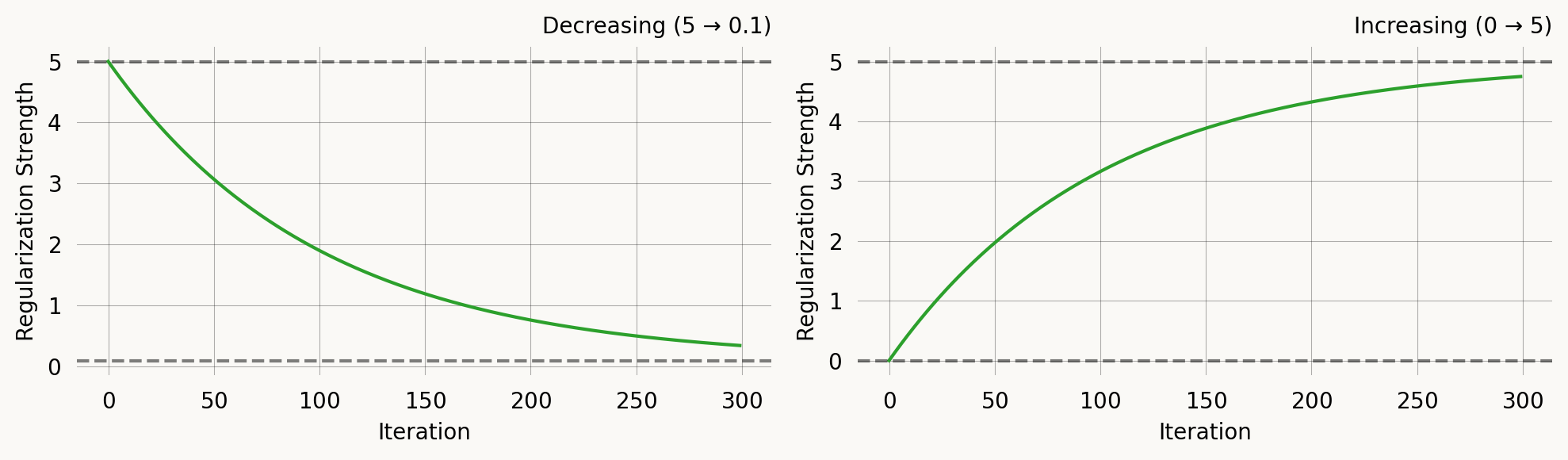

Se the API documentation for ExponentialCDFRegularization for all parameters.

Comparison

nr_iter = 300
iters = np.arange(nr_iter)

reg_schedules = {
    'Constant(1.0)': ConstantRegularization(1.0),
    'Exp(10 → 0.1, tau=50)': ExpRegularization(10.0, 0.1, 50.0),
    'ExpCDF(0 → 5, tau=100)': ExponentialCDFRegularization(0.0, 5.0, 100.0),
    'ExpCDF(5 → 0.1, tau=100)': ExponentialCDFRegularization(5.0, 0.1, 100.0),
}

fig, ax = plt.subplots(figsize=(7, 3))
for label, sched in reg_schedules.items():
    vals = [float(sched(i)) for i in iters]
    ax.plot(iters, vals, label=label)

ax.set_xlabel('Iteration')
ax.set_ylabel('Regularization Strength')
ax.set_title('Regularization schedules')
ax.legend(fontsize=8)
plt.tight_layout()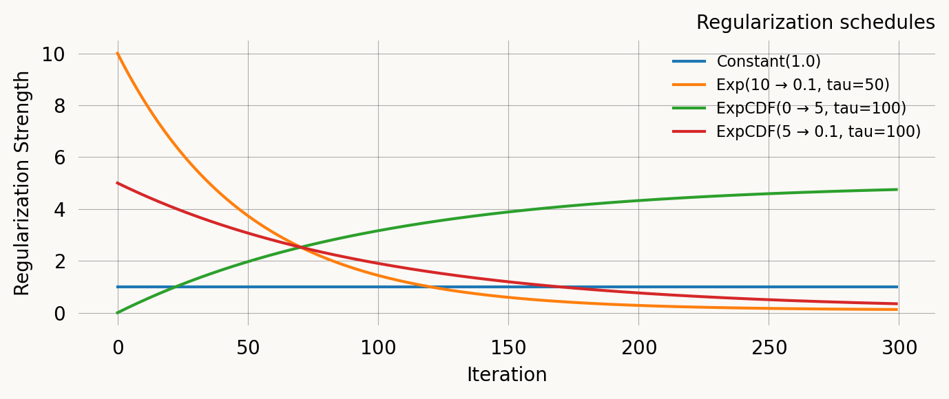

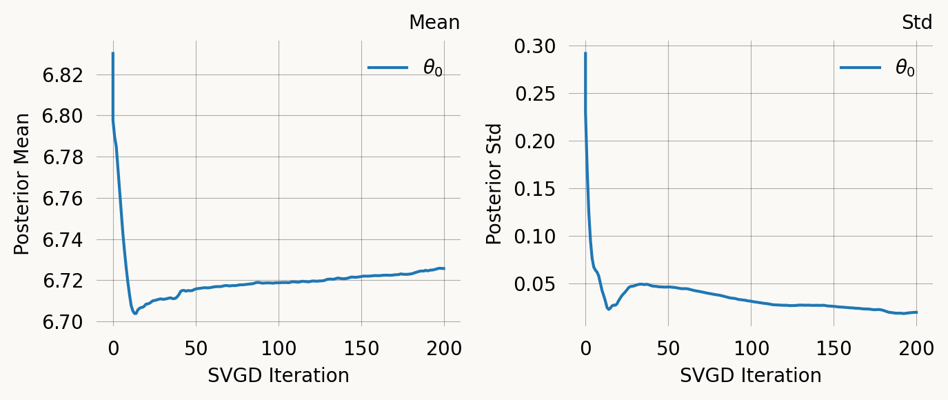
Putting it together

A typical SVGD call combining priors and schedules:

svgd = graph.svgd(
    data,
    prior=DataPrior(graph, data, sd=2.0),
    optimizer=Adam(
        learning_rate=ExpStepSize(first_step=0.1, last_step=0.01, tau=30.0),
    ),
    # regularization=ExpRegularization(first_reg=5.0, last_reg=0.1, tau=20.0),
    # nr_moments=2,
    n_iterations=200,
)
svgd.summary()
svgd.plot_convergence() ;

Parameter  Fixed      MAP        Mean       SD         HPD 95% lo   HPD 95% hi  
0          No         6.7210     6.7257     0.0198     6.6942       6.7676      

Particles: 24, Iterations: 200