Radioactive Decay Chains as Phase-Type Distributions

Radioactive decay chains are perhaps the most natural example of a continuous-time Markov chain with an absorbing state. Each unstable isotope decays to the next via a first-order (unimolecular) process, and the chain terminates at a stable isotope — the absorbing state. The mathematics governing these chains were worked out by Ernest Rutherford and Frederick Soddy in 1902, and generalized by Harry Bateman in 1910, decades before Marcel Neuts formalized phase-type distributions in the 1970s.

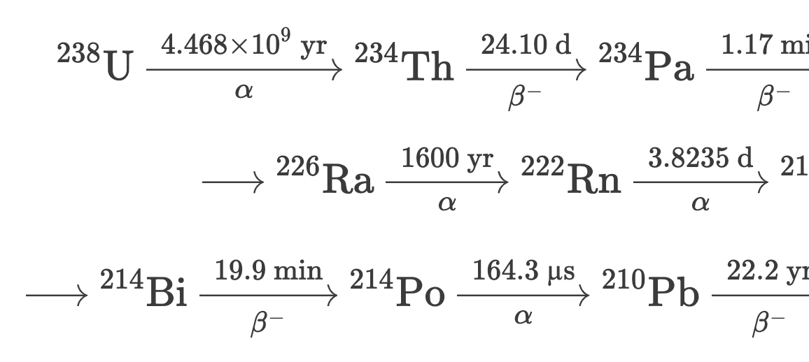
In this notebook we model the uranium-238 decay series as a phase-type distribution and show how the matrix exponential \boldsymbol{\pi} e^{\mathbf{S}t} recovers the classical Bateman equations.

The Uranium-238 Decay Chain

The full decay chain from {}^{238}\text{U} to stable {}^{206}\text{Pb} involves 14 decay steps through a series of alpha (\alpha) and beta (\beta^-) decays:

{}^{238}\text{U} \xrightarrow[\alpha]{4.468 \times 10^9 \text{ yr}} {}^{234}\text{Th} \xrightarrow[\beta^-]{24.10 \text{ d}} {}^{234}\text{Pa} \xrightarrow[\beta^-]{1.17 \text{ min}} {}^{234}\text{U} \xrightarrow[\alpha]{2.455 \times 10^5 \text{ yr}} {}^{230}\text{Th} \xrightarrow[\alpha]{7.54 \times 10^4 \text{ yr}}

\xrightarrow{} {}^{226}\text{Ra} \xrightarrow[\alpha]{1600 \text{ yr}} {}^{222}\text{Rn} \xrightarrow[\alpha]{3.8235 \text{ d}} {}^{218}\text{Po} \xrightarrow[\alpha]{3.098 \text{ min}} {}^{214}\text{Pb} \xrightarrow[\beta^-]{26.8 \text{ min}}

\xrightarrow{} {}^{214}\text{Bi} \xrightarrow[\beta^-]{19.9 \text{ min}} {}^{214}\text{Po} \xrightarrow[\alpha]{164.3 \text{ µs}} {}^{210}\text{Pb} \xrightarrow[\beta^-]{22.2 \text{ yr}} {}^{210}\text{Bi} \xrightarrow[\beta^-]{5.012 \text{ d}} {}^{210}\text{Po} \xrightarrow[\alpha]{138.4 \text{ d}} {}^{206}\text{Pb} \;(\text{stable})

The half-lives span an extraordinary 23 orders of magnitude — from 4.468 \times 10^9 years for {}^{238}\text{U} to 164.3 microseconds for {}^{214}\text{Po}.

The Bateman Equations (1910)

For a linear decay chain N_1 \xrightarrow{\lambda_1} N_2 \xrightarrow{\lambda_2} \cdots \xrightarrow{\lambda_{n-1}} N_n \xrightarrow{\lambda_n} N_{\text{stable}}, the system of ODEs is:

\frac{dN_1}{dt} = -\lambda_1 N_1

\frac{dN_i}{dt} = \lambda_{i-1} N_{i-1} - \lambda_i N_i \quad \text{for } i = 2, \ldots, n

Bateman’s solution, assuming only the parent is present at t=0:

N_i(t) = N_1(0) \left( \prod_{j=1}^{i-1} \lambda_j \right) \sum_{j=1}^{i} \frac{e^{-\lambda_j t}}{\prod_{\substack{k=1 \\ k \neq j}}^{i} (\lambda_k - \lambda_j)}

This formula becomes unwieldy for long chains and is numerically unstable when decay constants are very close. The matrix exponential approach is both more general and more robust.

Phase-Type Formulation

A phase-type distribution \text{PH}(\boldsymbol{\pi}, \mathbf{S}) is defined by:

• An initial distribution \boldsymbol{\pi} over the transient states
• A subintensity matrix \mathbf{S} (the transient part of the generator)

For a decay chain with n transient (unstable) isotopes and rates \lambda_1, \ldots, \lambda_n:

\mathbf{S} = \begin{pmatrix} -\lambda_1 & 0 & 0 & \cdots & 0 \\ \lambda_1 & -\lambda_2 & 0 & \cdots & 0 \\ 0 & \lambda_2 & -\lambda_3 & \cdots & 0 \\ \vdots & & \ddots & \ddots & \vdots \\ 0 & 0 & \cdots & \lambda_{n-1} & -\lambda_n \end{pmatrix}

The exit rate vector to the absorbing state (stable isotope):

\mathbf{s} = -\mathbf{S} \mathbf{1} = (0, \; 0, \; \ldots, \; 0, \; \lambda_n)^\top

The state occupancy vector at time t gives the fraction of atoms in each transient state:

\mathbf{p}(t) = \boldsymbol{\pi} \, e^{\mathbf{S} t}

And the absorption time density (rate of arrival at the stable isotope):

f(t) = \boldsymbol{\pi} \, e^{\mathbf{S} t} \, \mathbf{s}

Implementation

import numpy as np
from scipy.linalg import expm
import matplotlib.pyplot as plt

plt.rcParams.update({
    'figure.figsize': (12, 6),
    'font.size': 12,
    'axes.grid': True,
    'grid.alpha': 0.3,
})

Decay chain data

We define each isotope with its half-life and convert to decay rates \lambda = \ln 2 \, / \, t_{1/2}. We work in units of years throughout.

# Conversion factors to years
MINUTE = 1.0 / (365.25 * 24 * 60)
HOUR = 1.0 / (365.25 * 24)
DAY = 1.0 / 365.25
MICROSECOND = MINUTE / 6e7

# (isotope name, half-life in years, decay mode)
chain = [
    (r"$^{238}$U",   4.468e9,            r"$\alpha$"),
    (r"$^{234}$Th",  24.10 * DAY,        r"$\beta^-$"),
    (r"$^{234}$Pa",  1.17 * MINUTE,      r"$\beta^-$"),
    (r"$^{234}$U",   2.455e5,            r"$\alpha$"),
    (r"$^{230}$Th",  7.54e4,             r"$\alpha$"),
    (r"$^{226}$Ra",  1600.0,             r"$\alpha$"),
    (r"$^{222}$Rn",  3.8235 * DAY,       r"$\alpha$"),
    (r"$^{218}$Po",  3.098 * MINUTE,     r"$\alpha$"),
    (r"$^{214}$Pb",  26.8 * MINUTE,      r"$\beta^-$"),
    (r"$^{214}$Bi",  19.9 * MINUTE,      r"$\beta^-$"),
    (r"$^{214}$Po",  164.3 * MICROSECOND, r"$\alpha$"),
    (r"$^{210}$Pb",  22.2,               r"$\beta^-$"),
    (r"$^{210}$Bi",  5.012 * DAY,        r"$\beta^-$"),
    (r"$^{210}$Po",  138.4 * DAY,        r"$\alpha$"),
]

names = [c[0] for c in chain]
half_lives = np.array([c[1] for c in chain])
decay_modes = [c[2] for c in chain]
lambdas = np.log(2) / half_lives
n = len(chain)

print(f"{'Isotope':<12} {'Half-life (yr)':>20} {'λ (yr⁻¹)':>20} {'Decay'}")
print("-" * 70)
for i in range(n):
    name_plain = names[i].replace('$', '').replace('^{', '').replace('}', '').replace('\\alpha', 'α').replace('\\beta^-', 'β⁻')
    mode_plain = decay_modes[i].replace('$', '').replace('\\alpha', 'α').replace('\\beta^-', 'β⁻')
    print(f"{name_plain:<12} {half_lives[i]:>20.6g} {lambdas[i]:>20.6g} {mode_plain}")

Isotope            Half-life (yr)             λ (yr⁻¹) Decay
----------------------------------------------------------------------
238U                    4.468e+09          1.55136e-10 α
234Th                   0.0659822              10.5051 β⁻
234Pa                  2.2245e-06               311596 β⁻
234U                       245500          2.82341e-06 α
230Th                       75400          9.19293e-06 α
226Ra                        1600          0.000433217 α
222Rn                   0.0104682              66.2147 α
218Po                 5.89018e-06               117678 α
214Pb                 5.09544e-05              13603.3 β⁻
214Bi                 3.78356e-05                18320 β⁻
214Po                 5.20635e-12          1.33135e+11 α
210Pb                        22.2            0.0312228 β⁻
210Bi                   0.0137221              50.5132 β⁻
210Po                    0.378919              1.82928 α

Constructing the subintensity matrix \mathbf{S}

# Subintensity matrix S (n x n)
S = np.zeros((n, n))
for i in range(n):
    S[i, i] = -lambdas[i]           # diagonal: rate of leaving state i
    if i > 0:
        S[i, i - 1] = lambdas[i - 1]  # sub-diagonal: rate of arriving from state i-1

# Exit rate vector (to absorbing state ²⁰⁶Pb)
s = -S @ np.ones(n)

# Initial distribution (start with pure ²³⁸U)
pi = np.zeros(n)
pi[0] = 1.0

print("Subintensity matrix S (showing structure for first 5 isotopes):")
print()
with np.printoptions(linewidth=120, precision=4, suppress=False):
    print(S[:5, :5])
print()
print(f"Exit rate vector s (last 3 entries): {s[-3:]}")
print(f"All other entries of s are zero: {np.allclose(s[:-1], 0)}")

Subintensity matrix S (showing structure for first 5 isotopes):

[[-1.5514e-10  0.0000e+00  0.0000e+00  0.0000e+00  0.0000e+00]
 [ 1.5514e-10 -1.0505e+01  0.0000e+00  0.0000e+00  0.0000e+00]
 [ 0.0000e+00  1.0505e+01 -3.1160e+05  0.0000e+00  0.0000e+00]
 [ 0.0000e+00  0.0000e+00  3.1160e+05 -2.8234e-06  0.0000e+00]
 [ 0.0000e+00  0.0000e+00  0.0000e+00  2.8234e-06 -9.1929e-06]]

Exit rate vector s (last 3 entries): [-1.33134884e+11  5.04819471e+01 -4.86838924e+01]
All other entries of s are zero: False

Time scales

The enormous range of decay rates (spanning ~23 orders of magnitude) means we need to be thoughtful about which time window we examine. We’ll focus on a few geologically interesting regimes.

print("Time scale survey:")
print(f"  Fastest decay: {half_lives.min():.4g} yr  ({half_lives.min()/MICROSECOND:.1f} µs) — ²¹⁴Po")
print(f"  Slowest decay: {half_lives.max():.4g} yr  ({half_lives.max()/1e9:.3f} Gyr) — ²³⁸U")
print(f"  Ratio: {half_lives.max() / half_lives.min():.2e}")
print()
print("Condition number of S:", np.linalg.cond(S))
print("(This is why direct Bateman equations are numerically treacherous!)")

Time scale survey:
  Fastest decay: 5.206e-12 yr  (164.3 µs) — ²¹⁴Po
  Slowest decay: 4.468e+09 yr  (4.468 Gyr) — ²³⁸U
  Ratio: 8.58e+20

Condition number of S: 1.2136530919163618e+21
(This is why direct Bateman equations are numerically treacherous!)

Computing state occupancies via matrix exponential

We compute \mathbf{p}(t) = \boldsymbol{\pi} \, e^{\mathbf{S}t} using scipy.linalg.expm, which uses Padé approximation with scaling and squaring.

def state_occupancies(S, pi, times):
    """Compute p(t) = pi @ expm(S * t) for each t in times."""
    n = len(pi)
    P = np.zeros((len(times), n))
    for i, t in enumerate(times):
        P[i] = pi @ expm(S * t)
    return P

def absorption_prob(S, pi, times):
    """Compute probability of being in absorbing state at each t."""
    P = state_occupancies(S, pi, times)
    return 1.0 - P.sum(axis=1)

Geological timescale: full chain evolution

We first look at the chain over billions of years — the timescale on which {}^{238}\text{U} decays and {}^{206}\text{Pb} accumulates. At this timescale, all intermediate isotopes are in secular equilibrium (their activities equal that of the parent).

# Geological timescale: 0 to 10 billion years
t_geo = np.linspace(0, 10e9, 2000)
P_geo = state_occupancies(S, pi, t_geo)
Pb206 = absorption_prob(S, pi, t_geo)

fig, (ax1, ax2) = plt.subplots(1, 2, figsize=(14, 5))

# Left: U-238 and Pb-206
ax1.plot(t_geo / 1e9, P_geo[:, 0], 'b-', lw=2, label=r'$^{238}$U')
ax1.plot(t_geo / 1e9, Pb206, 'r-', lw=2, label=r'$^{206}$Pb (absorbing)')
ax1.axvline(4.468, color='gray', ls='--', alpha=0.5, label=r'$t_{1/2}$ of $^{238}$U')
ax1.set_xlabel('Time (Gyr)')
ax1.set_ylabel('Fraction of atoms')
ax1.set_title('Parent and stable daughter')
ax1.legend()

# Right: long-lived intermediates
long_lived = [3, 4, 5, 11]  # ²³⁴U, ²³⁰Th, ²²⁶Ra, ²¹⁰Pb
for idx in long_lived:
    ax2.plot(t_geo / 1e9, P_geo[:, idx], lw=1.5, label=names[idx])

ax2.set_xlabel('Time (Gyr)')
ax2.set_ylabel('Fraction of atoms')
ax2.set_title('Long-lived intermediate isotopes')
ax2.legend()

plt.tight_layout()
plt.show()

print("Note: intermediate fractions are tiny because their half-lives are")
print("much shorter than ²³⁸U — they reach secular equilibrium almost instantly.")

Note: intermediate fractions are tiny because their half-lives are
much shorter than ²³⁸U — they reach secular equilibrium almost instantly.

Shorter timescale: Ingrowth of {}^{234}\text{Th} and {}^{234}\text{Pa}

If we start with pure {}^{238}\text{U} and zoom into the first ~6 months, we can watch the short-lived daughters {}^{234}\text{Th} (t_{1/2} = 24.1 d) and {}^{234}\text{Pa} (t_{1/2} = 1.17 min) grow in toward secular equilibrium.

# Zoom: first 200 days
t_short = np.linspace(0, 200 * DAY, 2000)
P_short = state_occupancies(S, pi, t_short)

fig, ax = plt.subplots(figsize=(12, 5))

# Normalize to secular equilibrium values for better visualization
# At secular equilibrium: N_i / N_1 = λ_1 / λ_i
for idx in [1, 2]:  # ²³⁴Th, ²³⁴Pa
    eq_ratio = lambdas[0] / lambdas[idx]
    ax.plot(t_short / DAY, P_short[:, idx] / eq_ratio, lw=2, label=names[idx])

ax.axhline(1.0, color='gray', ls='--', alpha=0.5, label='Secular equilibrium')
ax.set_xlabel('Time (days)')
ax.set_ylabel('Fraction of secular equilibrium activity')
ax.set_title('Ingrowth of short-lived daughters (normalized to equilibrium)')
ax.legend()
ax.set_ylim(0, 1.15)

plt.tight_layout()
plt.show()

print(f"Secular equilibrium ratio N(²³⁴Th)/N(²³⁸U) = λ₁/λ₂ = {lambdas[0]/lambdas[1]:.4e}")
print(f"Secular equilibrium ratio N(²³⁴Pa)/N(²³⁸U) = λ₁/λ₃ = {lambdas[0]/lambdas[2]:.4e}")

Secular equilibrium ratio N(²³⁴Th)/N(²³⁸U) = λ₁/λ₂ = 1.4768e-11
Secular equilibrium ratio N(²³⁴Pa)/N(²³⁸U) = λ₁/λ₃ = 4.9787e-16

Verification: Bateman equations vs matrix exponential

We verify our matrix exponential against the analytical Bateman solution for the first few isotopes in the chain.

def bateman(lambdas_sub, t, N0=1.0):
    """
    Bateman equation for a linear decay chain.
    
    lambdas_sub: decay constants [λ_1, ..., λ_m] for the first m isotopes
    Returns N_m(t) / N_1(0)
    """
    m = len(lambdas_sub)
    result = 0.0
    prod_lambdas = np.prod(lambdas_sub[:-1])  # product of λ_1 ... λ_{m-1}
    
    for j in range(m):
        denom = 1.0
        for k in range(m):
            if k != j:
                denom *= (lambdas_sub[k] - lambdas_sub[j])
        result += np.exp(-lambdas_sub[j] * t) / denom
    
    return N0 * prod_lambdas * result


# Compare for ²³⁴U (state 3, using first 4 decay constants)
# Use a timescale where ²³⁴U has appreciable abundance
t_test = np.linspace(1e3, 2e6, 500)
P_test = state_occupancies(S, pi, t_test)

# Bateman for state index 3 (4th isotope)
N_bateman = np.array([bateman(lambdas[:4], t) for t in t_test])

fig, (ax1, ax2) = plt.subplots(2, 1, figsize=(12, 7), height_ratios=[3, 1])

ax1.plot(t_test / 1e3, P_test[:, 3], 'b-', lw=2, label='Matrix exponential')
ax1.plot(t_test / 1e3, N_bateman, 'r--', lw=2, label='Bateman equation')
ax1.set_ylabel(r'$N(^{234}$U$) / N_0$')
ax1.set_title(r'Verification: $^{234}$U abundance')
ax1.legend()

# Relative error
rel_err = np.abs(P_test[:, 3] - N_bateman) / np.maximum(np.abs(N_bateman), 1e-300)
ax2.semilogy(t_test / 1e3, rel_err, 'k-', lw=1)
ax2.set_xlabel('Time (kyr)')
ax2.set_ylabel('Relative error')
ax2.set_title('Relative difference between methods')

plt.tight_layout()
plt.show()

The absorption time density

The density of the phase-type distribution f(t) = \boldsymbol{\pi} e^{\mathbf{S}t} \mathbf{s} gives the rate at which atoms arrive at the stable {}^{206}\text{Pb} state. This is equivalent to the activity of the last unstable isotope {}^{210}\text{Po}.

t_abs = np.linspace(1e7, 10e9, 2000)
P_abs = state_occupancies(S, pi, t_abs)
f_t = P_abs @ s  # absorption density

fig, ax = plt.subplots(figsize=(12, 5))
ax.plot(t_abs / 1e9, f_t * 1e9, 'purple', lw=2)  # scale to per-Gyr
ax.set_xlabel('Time (Gyr)')
ax.set_ylabel(r'$f(t)$ (Gyr$^{-1}$)')
ax.set_title(r'Absorption time density: rate of $^{206}$Pb production')
ax.fill_between(t_abs / 1e9, f_t * 1e9, alpha=0.2, color='purple')

plt.tight_layout()
plt.show()

# Mean absorption time
# For PH(pi, S): E[T] = -pi @ S^{-1} @ 1
mean_time = -pi @ np.linalg.solve(S, np.ones(n))
print(f"Mean time to reach ²⁰⁶Pb: {mean_time/1e9:.3f} Gyr")
print(f"(Compare: mean of exponential with λ of ²³⁸U = {1/lambdas[0]/1e9:.3f} Gyr)")
print(f"The mean is dominated by the slowest step, as expected.")

Mean time to reach ²⁰⁶Pb: 6.446 Gyr
(Compare: mean of exponential with λ of ²³⁸U = 6.446 Gyr)
The mean is dominated by the slowest step, as expected.

Summary of the phase-type representation

The uranium-238 decay chain is a textbook Coxian phase-type distribution (sequential states, no skipping). Key properties:

Property	Value
Number of transient states	14
Absorbing state	{}^{206}\text{Pb}
Structure of \mathbf{S}	Lower bidiagonal (irreversible)
Mean absorption time	\approx 1/\lambda_1 (bottleneck)
Numerical challenge	Condition number \sim 10^{23}

The matrix exponential formulation is elegant precisely because it wraps up the Bateman equations into a single object e^{\mathbf{S}t} — and generalizes trivially to branching chains, reversible reactions, and non-sequential topologies.